Machine Learning
1.[ML] Decision Tree

개요분할변수와 분할점 결정분기마다 비용함수(불순도)가 가장 낮아지는 지점을 Grid Search를 통해 어떤 변수의 어떤 값을 기준으로 나눌지 정한다.불순도의 감소가 최대가 되도록 선택한다.비용함수2.1 Misclassification rate2.2 Gini Index
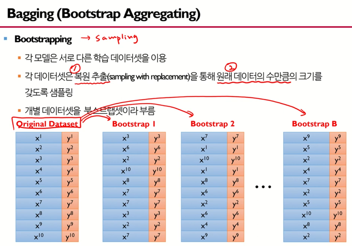
2.[Tree] Bagging - Random Forest
3.[ML] Boosting
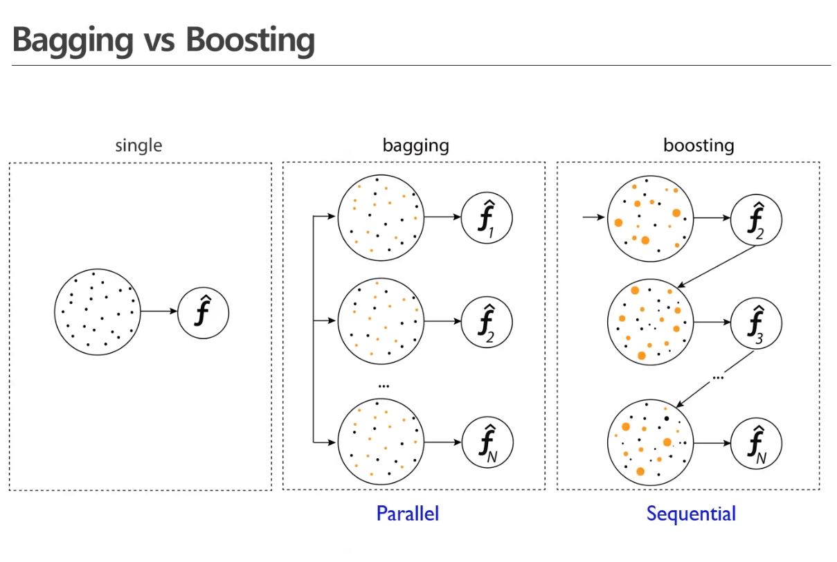
BOOSTINGIDEA: 여러개의 모델을 순차적으로 구축해서 최종적으로 합침각 단계에서 새로운 모델을 학습하여 이전 단계의 모델 단점을 보완알고리즘 종류Adaboost(Adaptive boosting)GBM(Gradient boosting machines)XGboost
4.[ML] Adaboost
AdaboostWeight > Total Error > Amount of Say > Weight update >> New Dataset based on the updated weights of the data > ...
5.[ML] Gradient Boosting Machine
GBMClassification: predicted probability(1st: log(odds)) > residual > updated predicted probability > residual > ...
6.[ML] XGBoost
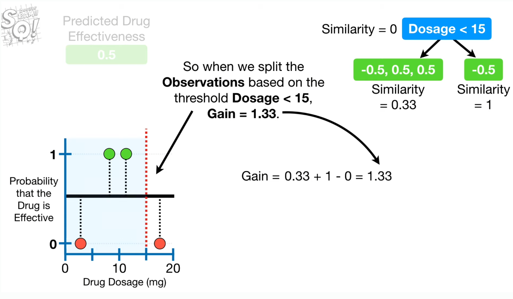
XGBoost병렬처리, 데이터를 구간화해서 효율적인 컴퓨팅오버피팅 방지: 정규화 추가 가능, 랜덤포레스트와 비슷하게 피처 일부를 무작위로 선택하여 학습.
7.[ML] Light Gradient Boosting Machine
Light Gradient Boosting MachineLevel-wise가 아닌 Leaf-wise로 진행전체 Loss가 줄어드는 방향으로 node를 선정해서 split 진행(이 때, level 유지하려는 경향을 포기)필요한 노드들만 dsplit하면 되기 때문에 lev
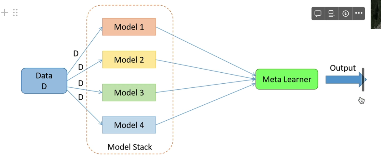
8.[ML] Stacking
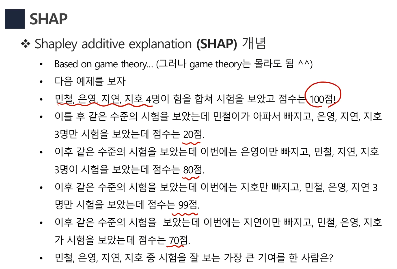
9.SHAP(Shaply additive explanation)
10.Association Rule
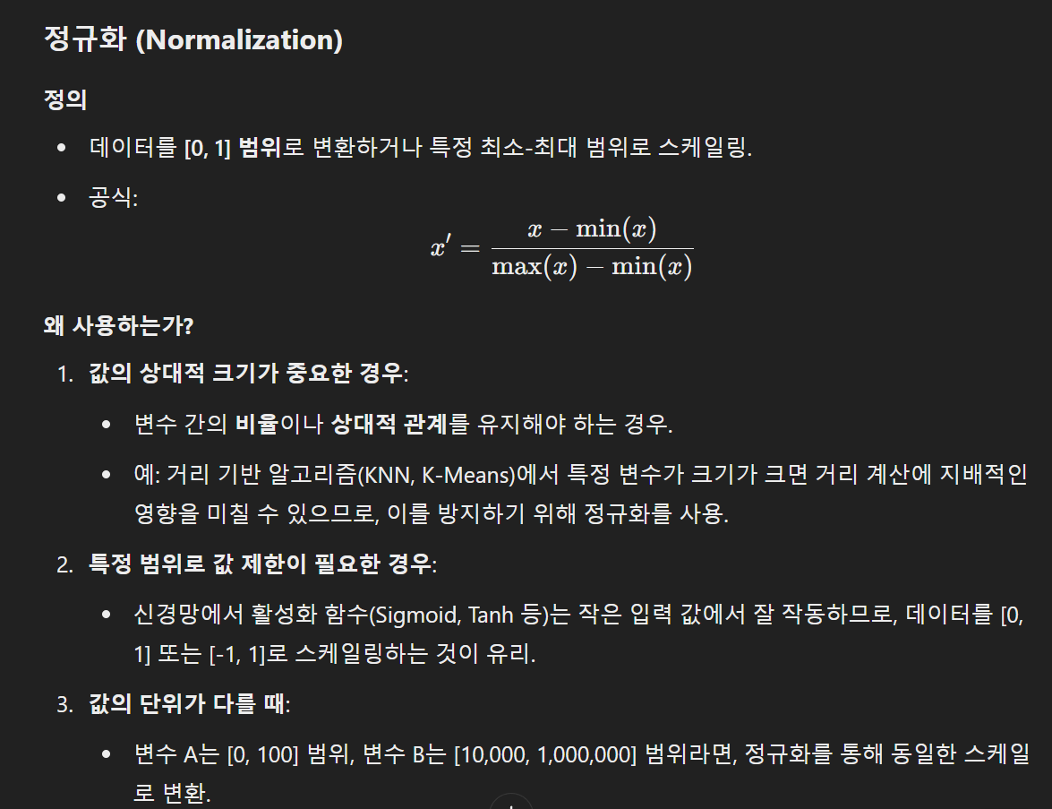
11.Normalization and Standardization
https://bskyvision.com/849
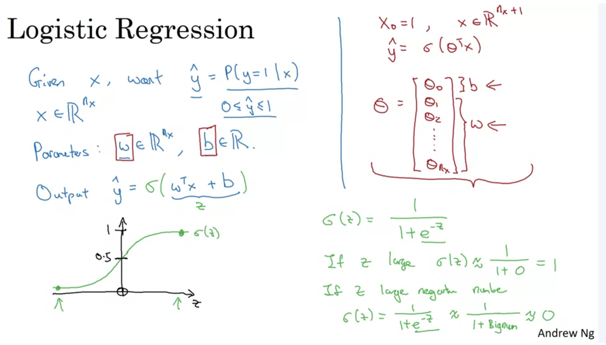
12.[ML] Logistic Regression
13.[DNN] Neural Network
Activation FunctionsHidden Layer의 Activation Function을 Linear Function으로 하면 Multi layer의 의미가 없어짐. 그래서 Non-linear function을 사용하는 것임.Random Initializati
14.[DNN] Activation Functions
Hidden Layer의 Activation Function을 Linear Function으로 하면 Multi layer의 의미가 없어짐. 그래서 Non-linear function을 사용하는 것임.Building blocks of DNNHyper-parametresL
15.[DNN, NN] Regularization
오버피팅을 방지하기 위한 조치로 L2 norm을 Cost Function에 더해줌. → 하이퍼파라미터인 lambda를 조정해야함.L2 Regularization이 가장 많이 사용됨.L1 Regularization을 사용하면 W matrix에 많은 숫자가 0이됨. 잘 사
16.[DNN] Weight Initialization
Zero Initializationa1과 a2가 완전히 동일한 output을 계산하게되므로 layer의 node를 여러개 두는게 의미가 없음.Random Initialization만약 Weight를 크게 설정하면 Sigmoid/Tanh function을 통과할 때 0
17.[DNN] Dropout Regularization
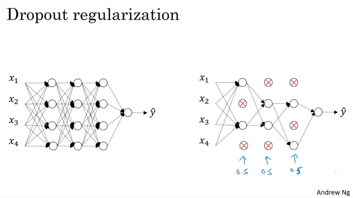
Using dropout, you can give the probability of keeping nodes to each layer. The most common way to implement this is Inverted dropout.Intuition: Can't
18.[DNN] Other Regularization Methods (Augmentation, Early Stopping)
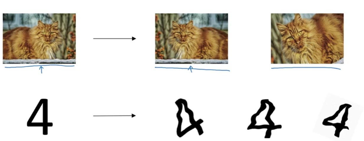
1\. Data augmentation2\. Early StoppingAs you train more the weights become bigger. So you stop in the middle, ideally when the dev set error is at th
19.[DNN] Normalizing inputs
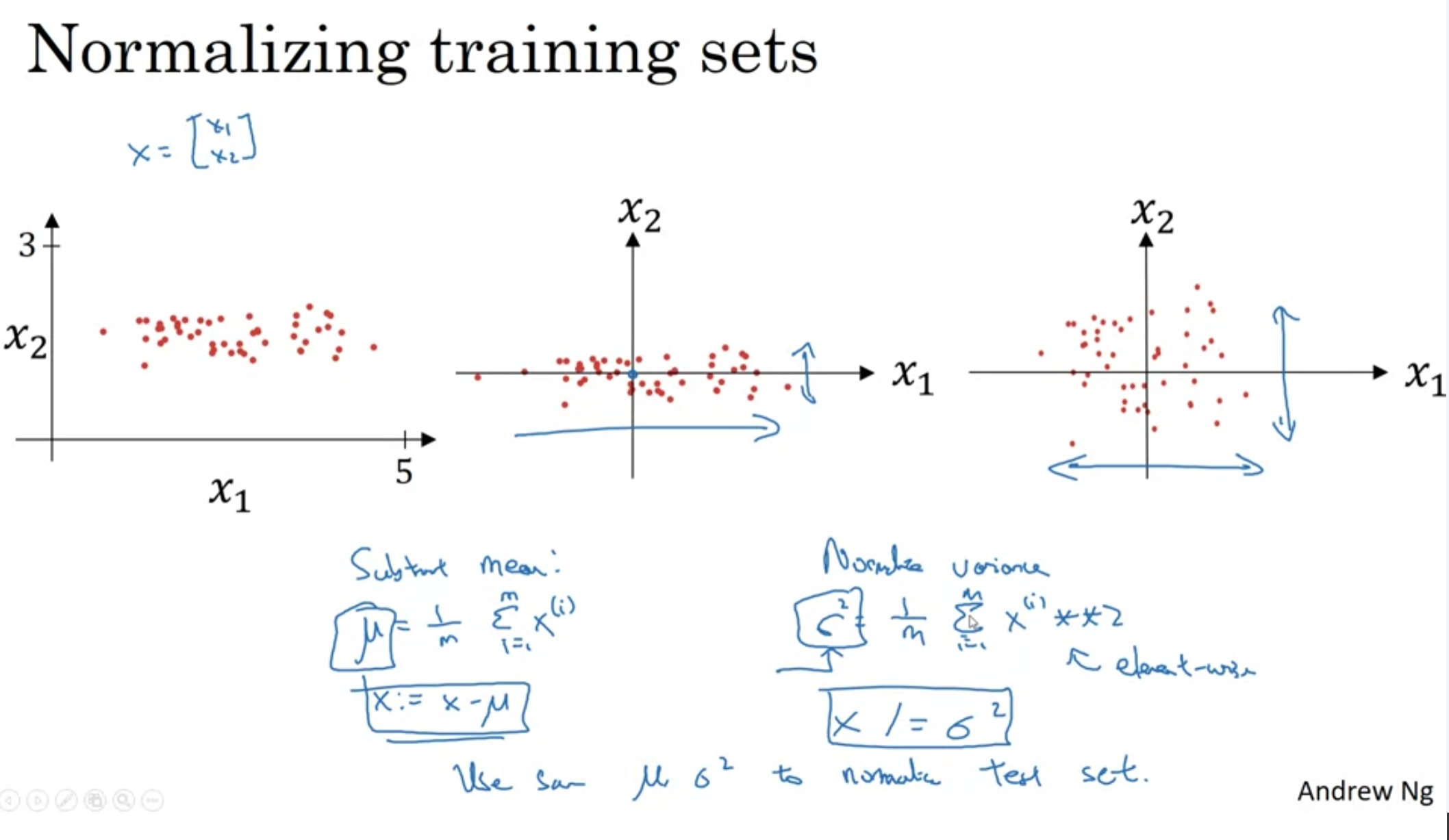
Normalizing inputsVanishing/exploding gradientsW가 1보다 크면 예측값이 너무 커지고W가 1보다 작으면 예측값이 너무 작아지는 현상?Weight initialization
20.[DNN] Vanishing/exploding gradients
Assume that b = 0 and we use linear activation functions throughout all the nodes.Then, y_hat becomes the multiplication of W matrices and the input m
21.[DNN] Gradient checking
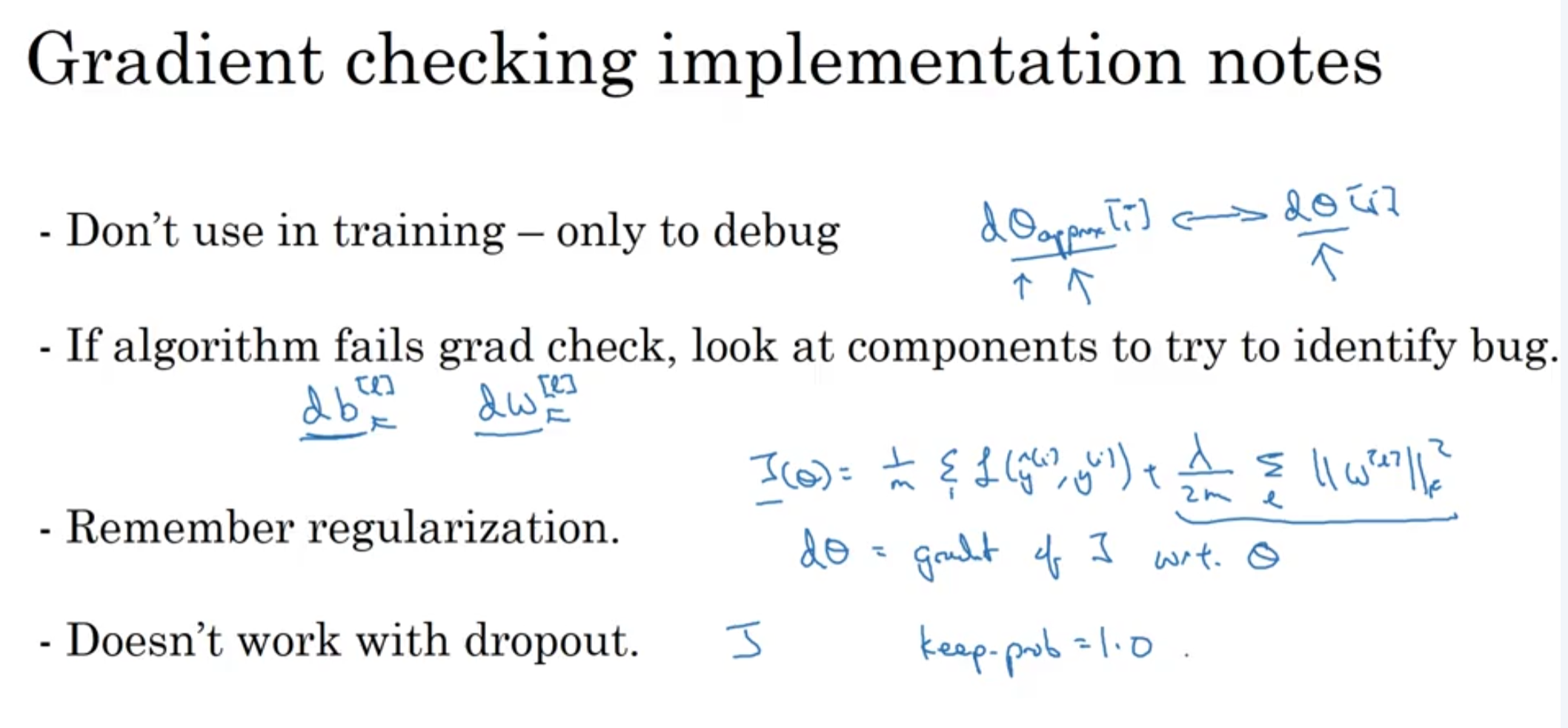
In backpropagation, you need to check if the values of the derivatives are correct.So you check the gradient using the technique of approximation in t
22.[DNN] Mini-batch gradient descent
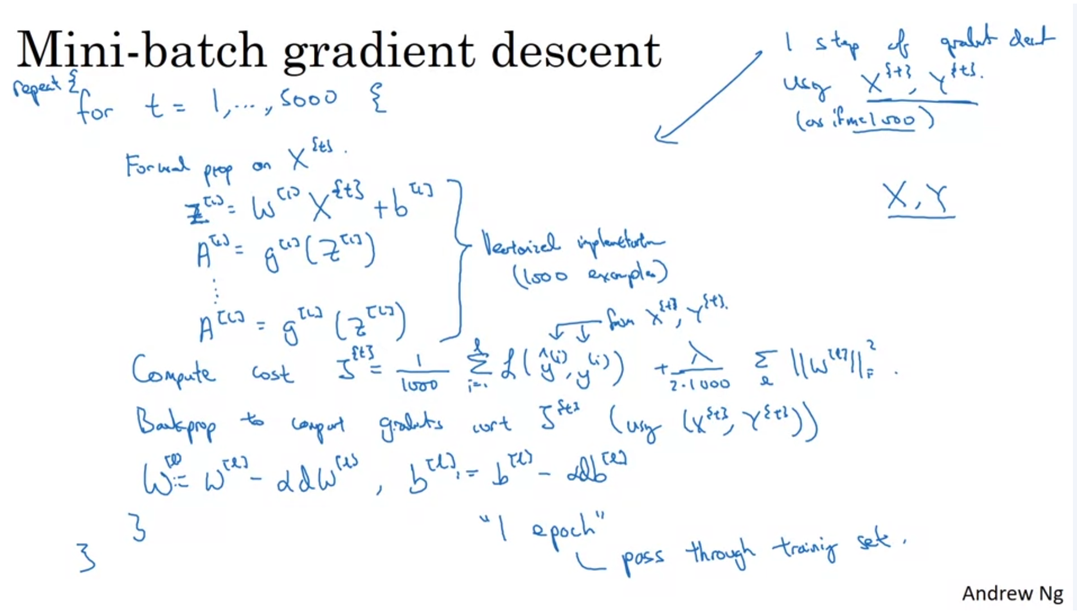
학습할 데이터가 많으면 mini-batch를 쓰는게 빠르고, minimum에 수렴할 가능성이 크다.
23.[DNN] Exponentially Weighted Moving Averages
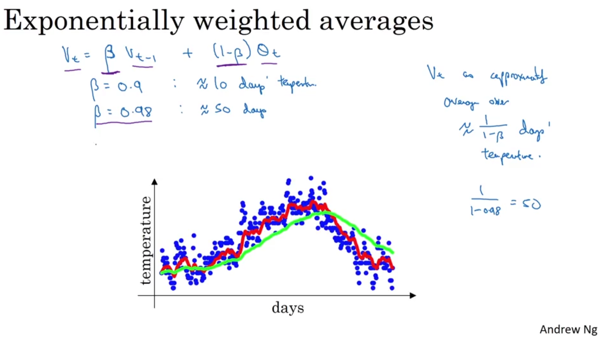
Beta 0.9(based on the past 10 days' temperature) > 붉은색Beta 0.98(based on the past 50 days' temperature) > 초록색주기를 더 짧게 잡을 수록 그래프의 fluctuation이 심해진다.Exp
24.[DNN] Gradient Descent with Momentum
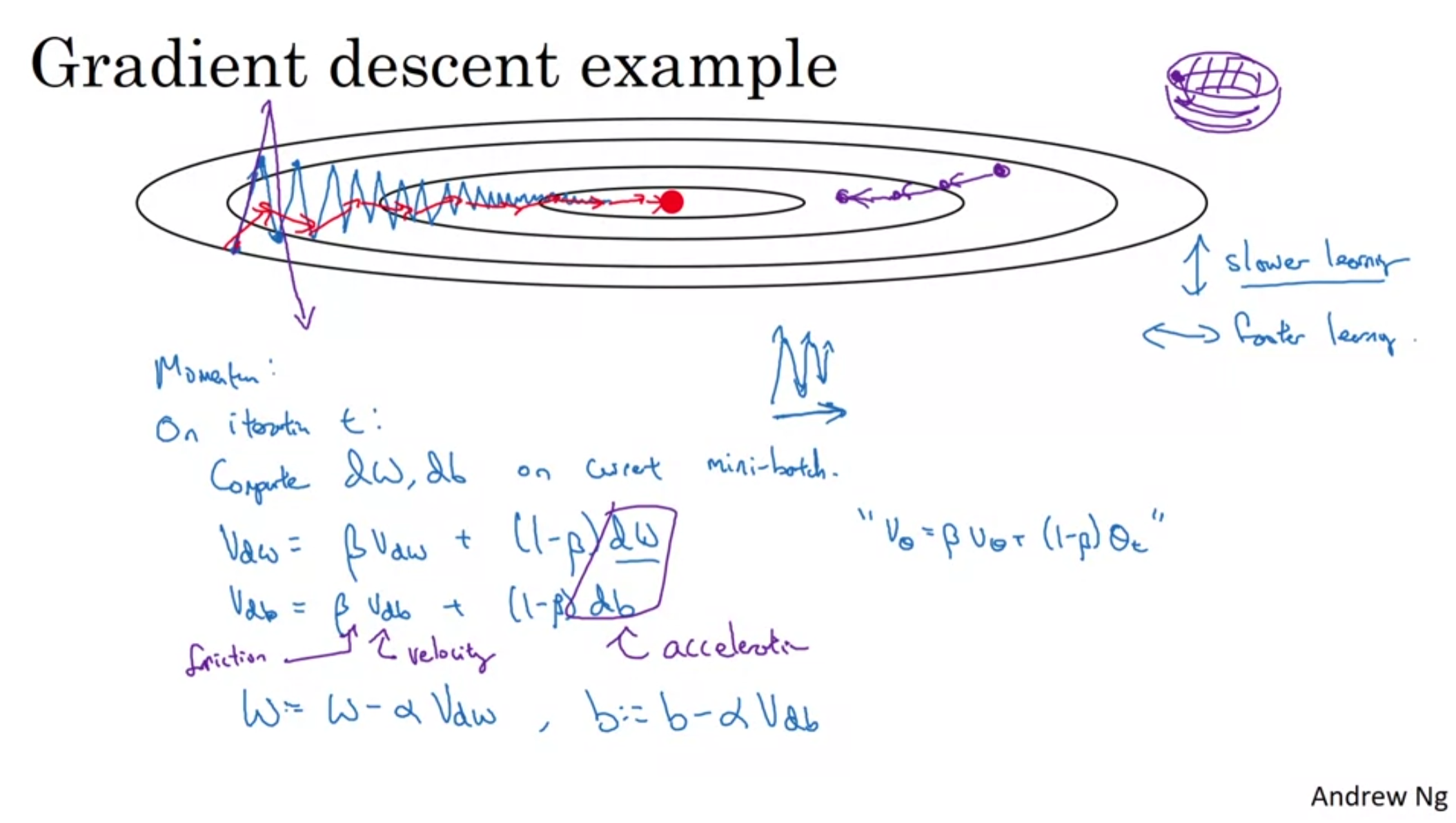
Gradient Descent with Momentum (moving weighted averages)RMS Prop Adam optimization = Momentum + RMSprop(Adaptive moment estimation)Learning rate deca
25.[DNN] RMS Prop
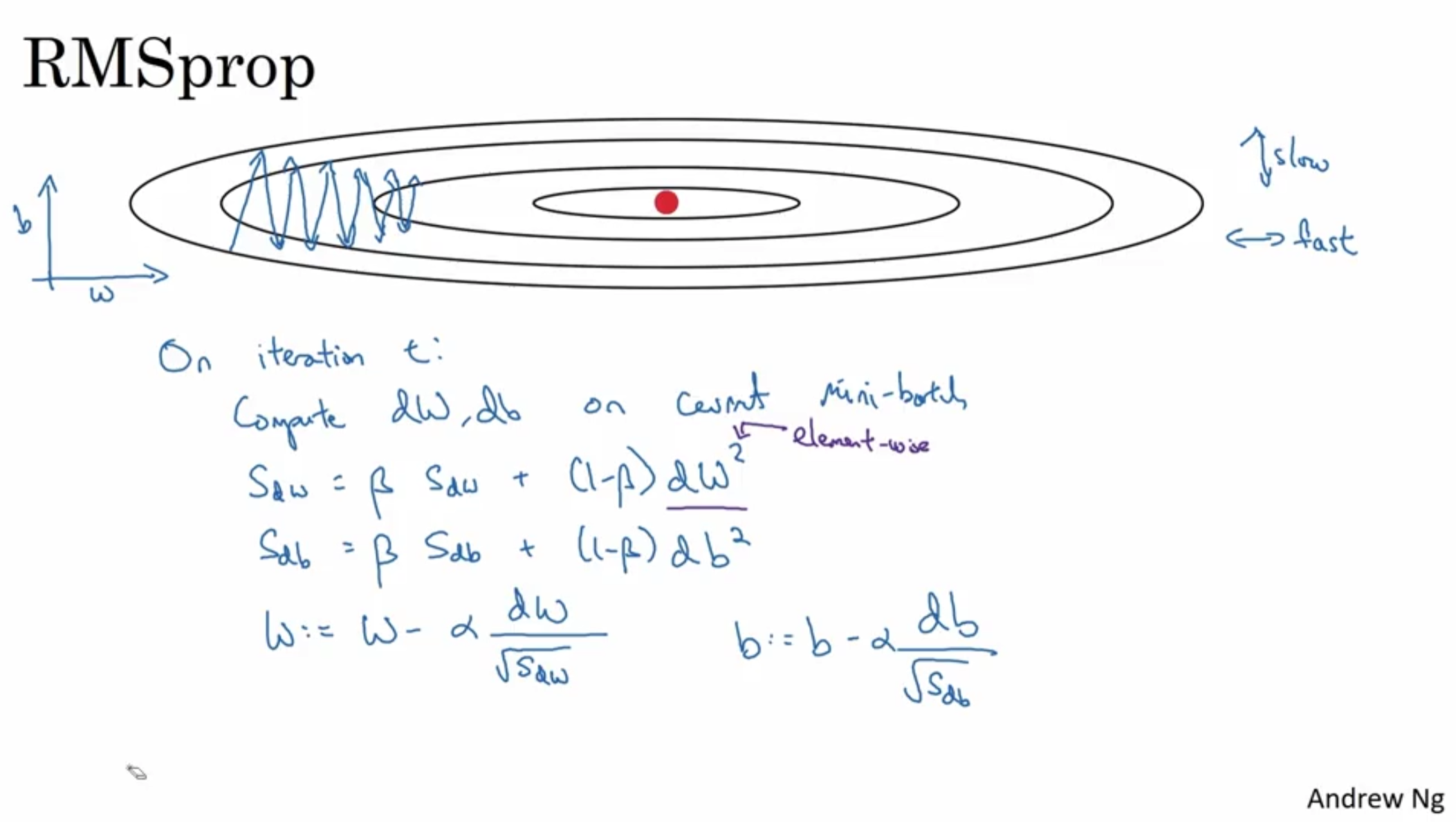
This is another way to speed up gradient descent.RMS Prop stands for Root Mean Squared propagation.Suppose in this example, w indicates the horizontal
26.[DNN] Adam optimization
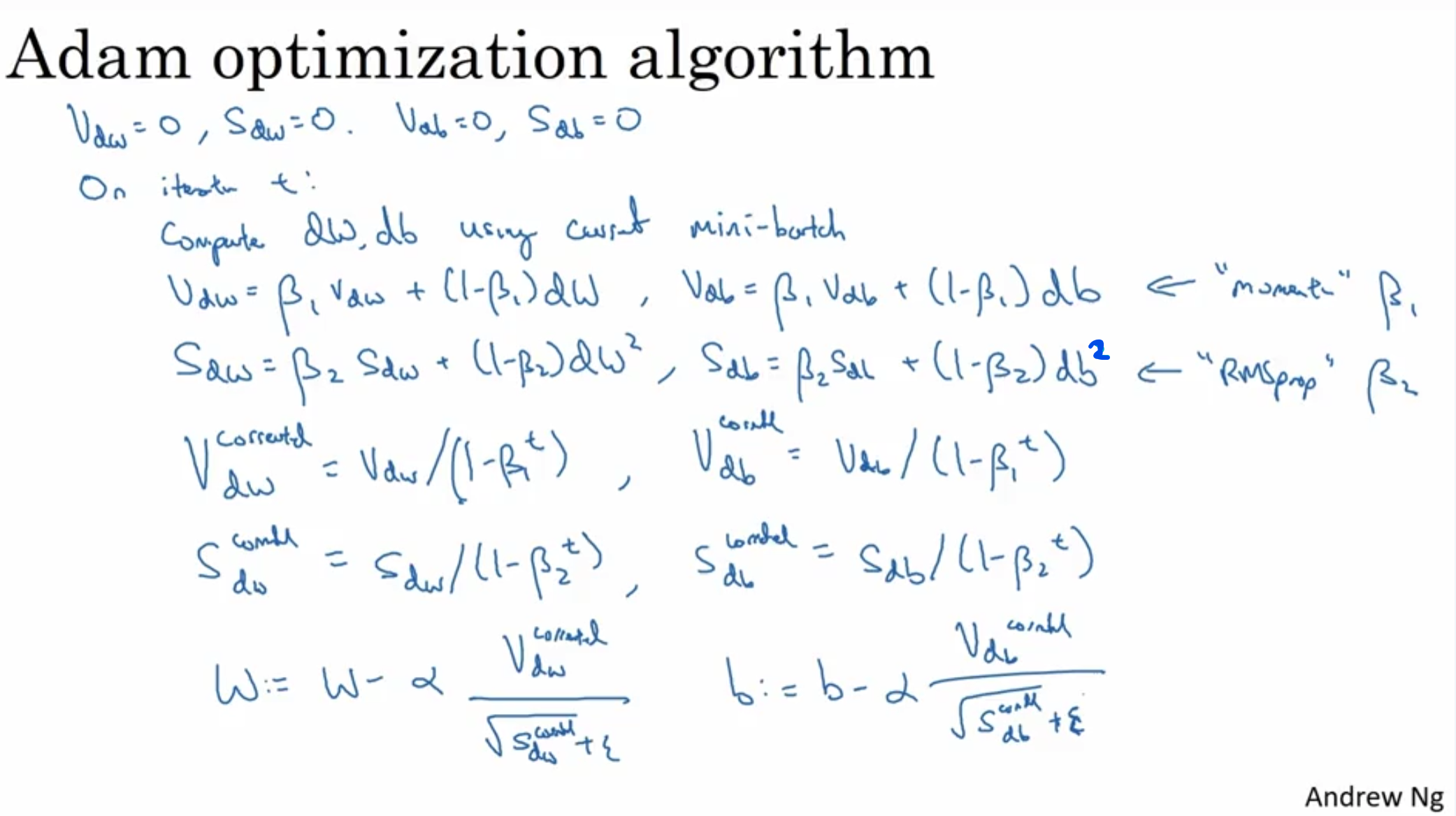
Adam optimization = Momentum + RMSprop(Adaptive moment estimation)Hyperparameters choice for Adam optimization (Recommendations)alpha : needs to be tu
27.[DNN] Learning Rate Dacay
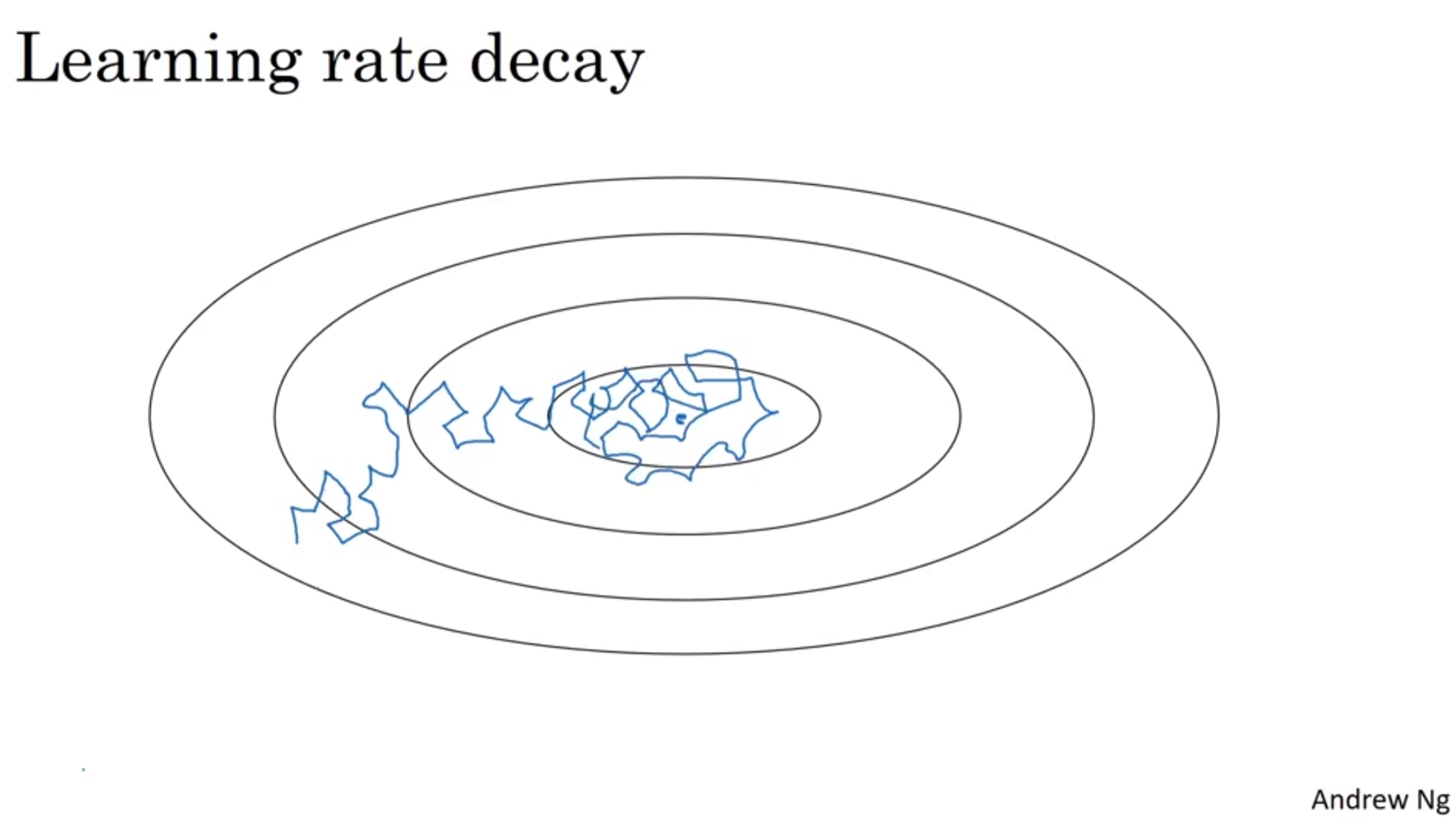
Learning rate decayAnother way to speed up the learning algorithm is to slowly reduce the learning rate over time.If the learning rate is fixed over a
28.[DNN] The problem of Local Optima
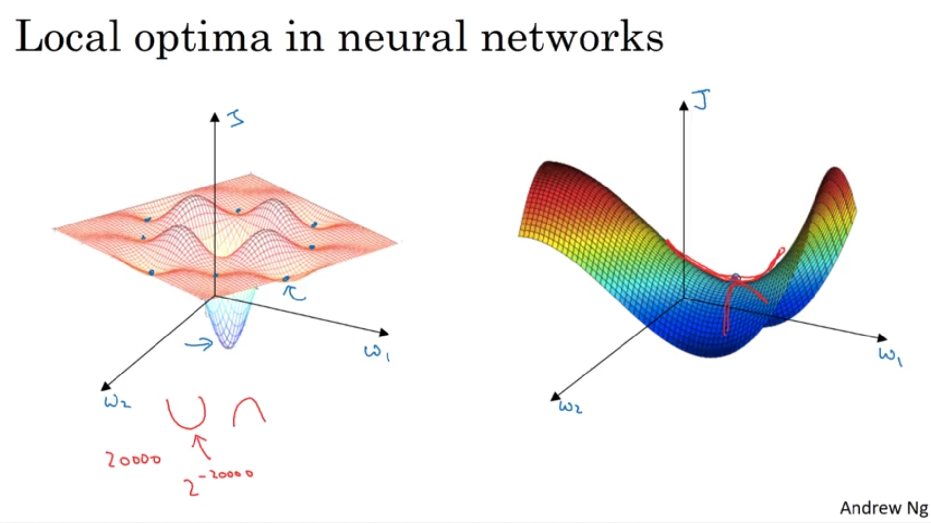
(Left) 과거에 Neural Network에서 gradient가 0인 구간에 빠지는 현상을 local optima라고 표현했다.(Right) 하지만 실제로 gradient가 0이되는 구간은 local optima 보다 saddle point인 경우가 대부분이다.
29.[DNN] Hyperparametre Tuning
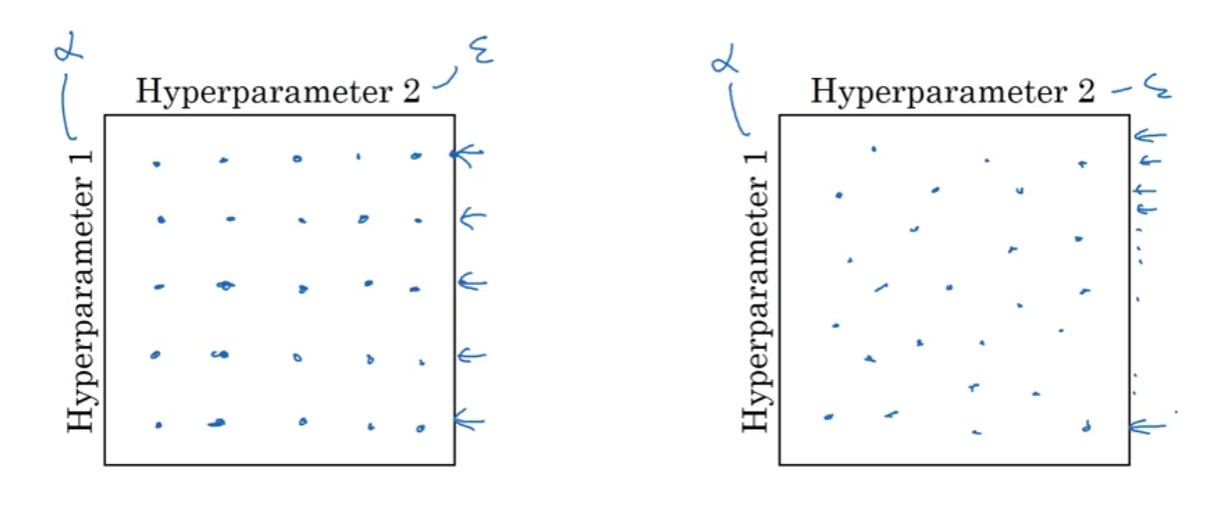
Hyperparametres to tune in order of importanceLearning rate(alpha)Momentum(Beta) - recomm: 0.9Number of Hidden UnitsMini-batch sizeNumber of LayersLea
30.[DNN] Batch Normalization
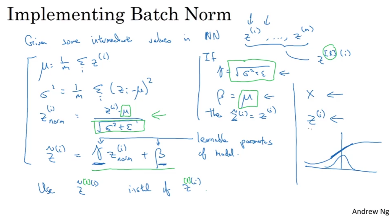
In logistic regression, normalizing INPUT FEATURES speeds up learning.In deep learning, for any hidden layer, can we normalize the activation function