스터디노트 (DeepLearning 11)

Transfer Learning - 전이학습과 미세조정

• tensorflow

from __future__ import absolute_import, division, print_function, unicode_literals

import os
import numpy as np
import matplotlib.pyplot as plt
import tensorflow as tf

keras = tf.keras

# tfds를 통해 데이터를 가져올 준비

import tensorflow_datasets as tfds

tfds.disable_progress_bar()

# 데이터 받기

(raw_train, raw_validation, raw_test), metadata = tfds.load(
    'cats_vs_dogs', split=['train[:80%]', 'train[80%:90%]', 'train[90%:]'],
    with_info=True,
    as_supervised=True,
)
# as_supervised 옵션을 True로 하면 데이터가 라벨과 함께 tuple 형태로 저장됨

# 데이터 탐색

for image, label in raw_train.take(1):
  plt.imshow(image)
  print(label.numpy())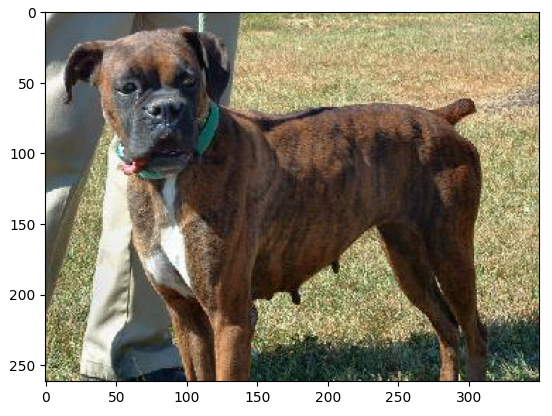

# 메타 정보에서 라벨 이름 가져와서 두 개만

get_label_name = metadata.features['label'].int2str

for image, label in raw_train.take(2):
  plt.figure()
  plt.imshow(image)
  plt.title(get_label_name(label))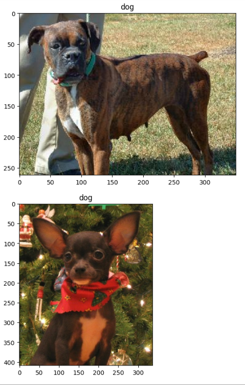

# 이미지 전처리 함수

IMG_SIZE = 160 # 모든 이미지 160 * 160

def format_example(image, label):
  image = tf.cast(image, tf.float32)
  image = (image/127.5) - 1 # -1 ~ 1 사이의 값으로 변경
  image = tf.image.resize(image, (IMG_SIZE, IMG_SIZE))
  return image, label

# map 함수를 이용해서 적용

train = raw_train.map(format_example)
validation = raw_validation.map(format_example)
test = raw_test.map(format_example)

# batch size 적용하고 shuffle

BATCH_SIZE = 32
SHUFFLE_BUFFER_SIZE = 1000

train_batches = train.shuffle(SHUFFLE_BUFFER_SIZE).batch(BATCH_SIZE)
validation_batches = validation.batch(BATCH_SIZE)
test_batches = test.batch(BATCH_SIZE)

# 확인

for image_batch, label_batch in train_batches.take(1):
  pass
image_batch.shape # batch size 설정한 값, 해상도 값

# MobileNet V2 모델
# 1.4M 이미지와 1000개의 클래스로 구성된 대규모 데이터셋인 ImageNet 데이터 셋을 사용해 사전 훈련된 모델
# 먼저 기능 추출에 사용할 MobileNet V2 층을 선택
# flatten 연산을 하기 전에 맨 아래 층을 가지고 진행(병목층)
# include_top = False로 지정하면 맨 위에 분류 층이 포함되지 않은 네트워크를 로드하므로 특징 추출에 이상적


IMG_SHAPE = (IMG_SIZE, IMG_SIZE, 3)

base_model = tf.keras.applications.MobileNetV2(input_shape = IMG_SHAPE,
                                               include_top = False,
                                               # include_top = False : 출력단을 말함, 이걸 빼고 가지고 와라라는 것을 의미
                                               weights = 'imagenet')

# feature_batch
# 이 특징 추출기는 각 160*160*3 이미지를 5*5*1280 개의 특징 블록으로 변환
# 1280 : 채널의 수

feature_batch = base_model(image_batch)
print(feature_batch.shape)

# 모델 확인

base_model.trainable = False

base_model.summary()

# GlobalAveragePooling2D 층을 사용하여 특징을 이미지 한개 당 1280개의 요소 벡터로 변환

global_average_layer = tf.keras.layers.GlobalAveragePooling2D()
feature_batch_average = global_average_layer(feature_batch)
print(feature_batch_average.shape)

# Dense층을 사용하여 특징을 이미지당 단일 예측
# 1 : 강아지, 0 : 고양이
prediction_layer = keras.layers.Dense(1)
prediction_batch = prediction_layer(feature_batch_average)
print(prediction_batch.shape)

# 양수는 클래스 1을 예측하고 음수는 클래스 0을 예측

prediction_batch

# 전체 모델 구성

model = tf.keras.Sequential([base_model,
                             global_average_layer,
                             prediction_layer])

# 모델 컴파일

base_learning_rate = 0.0001
model.compile(optimizer=tf.keras.optimizers.RMSprop(lr=base_learning_rate),
              loss = tf.keras.losses.BinaryCrossentropy(from_logits=True),
              metrics=['accuracy'])

# 모델 summary

model.summary()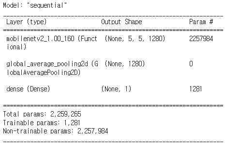

# 아무 학습을 하지 않은 현재의 성능

initial_epochs = 10
validation_steps = 20

loss0, accuracy0 = model.evaluate(validation_batches, steps=validation_steps)

# 학습
# trainable weights가 1200여개뿐이지만 연산은 전체를 다해야 하기 때문에 시간이 소요됨
# 그러나 mobilenet 전체를 다시 학습하는 것보다는 훨씬 좋음

history = model.fit(train_batches,
                    epochs=initial_epochs,
                    validation_data = validation_batches)

# 곡선이 예쁘게 수렴하긴 했는데

acc = history.history['accuracy']
val_acc = history.history['val_accuracy']

loss = history.history['loss']
val_loss = history.history['val_loss']

plt.figure(figsize=(8, 8))
plt.subplot(2, 1, 1)
plt.plot(acc, label='Training Accuracy')
plt.plot(val_acc, label='Validation Accuracy')
plt.legend(loc='lower right')
plt.ylabel('Accuracy')
plt.ylim([min(plt.ylim()), 1])
plt.title('Training and Validation Accuracy')

plt.subplot(2, 1, 2)
plt.plot(loss, label='Training Loss')
plt.plot(val_loss, label='Validation Loss')
plt.legend(loc='upper right')
plt.ylabel('Cross Entropy')
plt.ylim([0, 1])
plt.title('Training and Validation Loss')
plt.xlabel('epoch')
plt.show()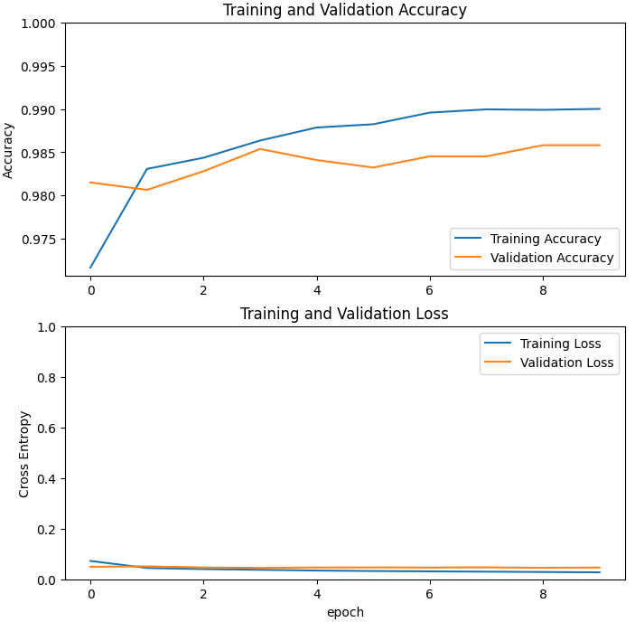

# 일단 모두 tarinable하게 변경

base_model.trainable = True
print('Number of layers in the base model : ', len(base_model.layers))

# 100번째 층부터 튜닝가능하게 설정

fine_tune_at = 100

# fine_tune_at 층 이전의 모든 층을 고정

for layer in base_model.layers[:fine_tune_at]:
  layer.trainable = False

# 학습 비율을 낮춤

model.compile(loss=tf.keras.losses.BinaryCrossentropy(from_logits=True),
              optimizer = tf.keras.optimizers.RMSprop(lr=base_learning_rate/10),
              metrics=['accuracy'])

model.summary()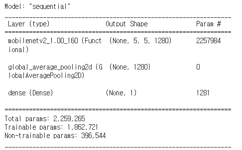

# 시작이 1 epoch가 아니다


fine_tune_epochs = 10
total_epochs = initial_epochs + fine_tune_epochs

history_fine = model.fit(train_batches,
                         epochs=total_epochs,
                         initial_epoch = history.epoch[-1], # 앞에 이어서 학습
                         validation_data=validation_batches)

# 최초 history에 방금 학습 결과를 추가

acc += history_fine.history['accuracy']
val_acc += history_fine.history['val_accuracy']

loss += history_fine.history['loss']
val_loss += history_fine.history['val_loss']

# 그래프

plt.figure(figsize=(8, 8))
plt.subplot(2, 1, 1)
plt.plot(acc, label='Training Accuracy')
plt.plot(val_acc, label='Validation Accuracy')
plt.ylim([0.8, 1])
plt.plot([initial_epochs-1, initial_epochs-1], plt.ylim(), label='Start Fine Tuning')
plt.legend(loc='lower right')
plt.title('Training and Validation Accuracy')

plt.subplot(2, 1, 2)
plt.plot(loss, label='Training Loss')
plt.plot(val_loss, label='Validation Loss')
plt.ylim([0, 1])
plt.plot([initial_epochs-1, initial_epochs-1], plt.ylim(), label='Start Fine Tuning')
plt.legend(loc='upper right')
plt.title('Training and Validation Loss')
plt.xlabel('epoch')
plt.show()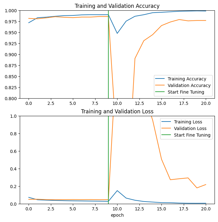

예상과 다르게 그래프가 그려졌는데...너무너무 어렵다 ㅠㅠ..
💻 출처 : 제로베이스 데이터 취업 스쿨