스터디노트 (DeepLearning 12)

Transfer Learning - 전이학습과 미세조정 - 꽃이름 맞추기

# 텐서플로 허브
# import, 설치

import matplotlib.pylab as plt
import tensorflow as tf

!pip install -U tf-hub-nightly

import tensorflow_hub as hub
from tensorflow.keras import layers

# 텐서플로 허브에서 mobilenet 가져오기

url = 'https://tfhub.dev/google/tf2-preview/mobilenet_v2/classification/2'
classifier_url = url

IMAGE_SHAPE = (224, 224)

classifier = tf.keras.Sequential([
hub.KerasLayer(classifier_url, input_shape=IMAGE_SHAPE + (3, ))
])

classifier.summary()

# 이미지 하나 가져와보기

import numpy as np
import PIL.Image as Image

url = 'https://storage.googleapis.com/download.tensorflow.org/example_images/grace_hopper.jpg'
grace_hopper = tf.keras.utils.get_file('image.jpg', url)
grace_hopper = Image.open(grace_hopper).resize(IMAGE_SHAPE)
grace_hopper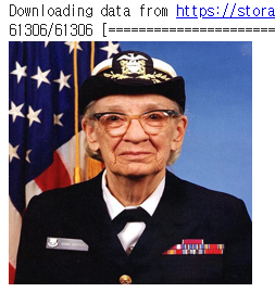

# 정규화

grace_hopper = np.array(grace_hopper)/255
grace_hopper.shape

# 예측

result = classifier.predict(grace_hopper[np.newaxis, ...])
result.shape

# argmax로 인덱스 찾기

predicted_class = np.argmax(result[0], axis=-1) # 원핫인코딩때문에 index를 읽기 위하여 
predicted_class

# label 받기

url = 'https://storage.googleapis.com/download.tensorflow.org/data/ImageNetLabels.txt'
labels_path = tf.keras.utils.get_file('ImageNetLabels.txt', url)
imagenet_labels = np.array(open(labels_path).read().splitlines())

# 확인

plt.imshow(grace_hopper)
plt.axis('off')
predicted_class_name = imagenet_labels[predicted_class]
_ = plt.title('Prediction : ' + predicted_class_name.title())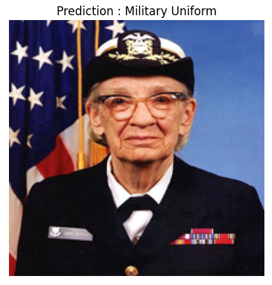

# 꽃

url = 'https://storage.googleapis.com/download.tensorflow.org/example_images/flower_photos.tgz'
data_root = tf.keras.utils.get_file(
    'flower_photos', url,
    untar=True)

# rescale 및 라벨 인식

image_generator = tf.keras.preprocessing.image.ImageDataGenerator(rescale=1/255)
image_data = image_generator.flow_from_directory(str(data_root), target_size=IMAGE_SHAPE)

# image_batch 생성

for image_batch, label_batch in image_data:
  print('Image batch shape : ', image_batch.shape)
  print('Label batch shape : ', label_batch.shape)
  break

# 배치한 셋에 대한 예측 결과

result_batch = classifier.predict(image_batch) # classifier : 현재는 imagenet기준으로 학습한 분류기
result_batch.shape

predicted_class_name = imagenet_labels[np.argmax(result_batch, axis=-1)]
predicted_class_name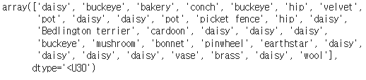

# 확인

plt.figure(figsize=(10, 9))
plt.subplots_adjust(hspace=0.5)
for n in range(30):
  plt.subplot(6, 5, n+1)
  plt.imshow(image_batch[n])
  plt.title(predicted_class_name[n])
  plt.axis('off')
_ = plt.suptitle('ImageNet predictions')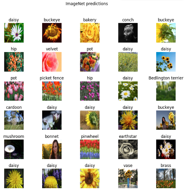

# 다시 특징 추출기

feature_extractor_url = 'https://tfhub.dev/google/tf2-preview/mobilenet_v2/feature_vector/2'

feature_extractor_layer = hub.KerasLayer(feature_extractor_url, input_shape=(224, 224, 3))

feature_batch = feature_extractor_layer(image_batch)
print(feature_batch.shape)

# dense 레이어 추가

feature_extractor_layer.trainable = False

model = tf.keras.Sequential([
    feature_extractor_layer,
    layers.Dense(image_data.num_classes, activation='softmax') # 내 라벨에 맞춰서 추가
])

model.summary()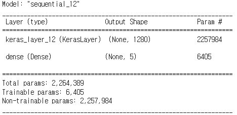

# 마지막 층

predictions = model(image_batch)

predictions.shape

# 컴파일

model.compile(
    optimizer=tf.keras.optimizers.Adam(),
    loss = 'categorical_crossentropy', metrics=['acc'])

# callback 하나 정의

class CollectBatchStats(tf.keras.callbacks.Callback):
  def __init__(self):
    self.batch_losses = []
    self.batch_acc = []
  
  def on_train_batch_end(self, batch, logs=None): # loss, acc 배치별로 뽑아줌
    self.batch_losses.append(logs['loss'])
    self.batch_acc.append(logs['acc'])
    self.model.reset_metrics()

# 학습

steps_per_epoch = np.ceil(image_data.samples/image_data.batch_size)

batch_stats_callback = CollectBatchStats()

history = model.fit_generator(image_data, epochs = 2,
                              steps_per_epoch=steps_per_epoch,
                              callbacks = [batch_stats_callback])

# loss는 떨어짐

plt.figure()
plt.ylabel('Loss')
plt.xlabel('Training Steps')
plt.ylim([0, 2])
plt.plot(batch_stats_callback.batch_losses)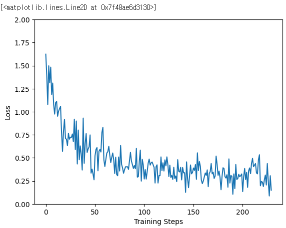

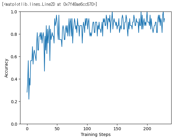
# acc는 잘됨

plt.figure()
plt.ylabel('Accuracy')
plt.xlabel('Training Steps')
plt.ylim([0, 1])
plt.plot(batch_stats_callback.batch_acc)

# class name 할당

class_names = sorted(image_data.class_indices.items(), key=lambda pair:pair[1])
class_names = np.array([key.title() for key, value in class_names]) # 원래 라벨..?
class_names

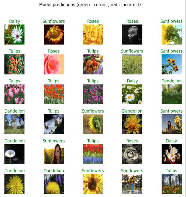
# 다시 예측

predicted_batch = model.predict(image_batch)
predicted_id = np.argmax(predicted_batch, axis = -1)
predicted_label_batch = class_names[predicted_id]


label_id = np.argmax(label_batch, axis = -1)

# 다시 확인

plt.figure(figsize=(10, 9))
plt.subplots_adjust(hspace=0.5)
for n in range(30):
  plt.subplot(6, 5, n+1)
  plt.imshow(image_batch[n])
  color = 'green' if predicted_id[n] == label_id[n] else 'red'
  plt.title(predicted_label_batch[n].title(), color = color)
  plt.axis('off')
_ = plt.suptitle('Model predictions (green : correct, red : incorrect)')

# 모델 저장하기

import time
t = time.time()

export_path = './{}'.format(int(t))
model.save(export_path, save_format = 'tf')

export_path

# 다시 모델 읽기

reloaded = tf.keras.models.load_model(export_path)

result_batch = model.predict(image_batch)
reloaded_result_batch = reloaded.predict(image_batch)

abs(reloaded_result_batch - result_batch).max()

너무너무 어렵다 ㅠㅠ...
💻 출처 : 제로베이스 데이터 취업 스쿨