Body Performance Data
데이터 출처
This is data that confirmed the grade of performance with age and some exercise performance data.
데이터는 총 12개의 칼럼과 13393개의 rows로 구성
| Header | Description |
|---|---|
| age | 20 ~64 |
| gender | F,M |
| height_cm | - |
| weight_kg | - |
| body fat_% | - |
| diastolic | diastolic blood pressure (min) |
| systolic | systolic blood pressure (min) |
| gripForce | - |
| sit and bend forward_cm | - |
| sit-ups counts | - |
| broad jump_cm | - |
| class | A,B,C,D ( A: best) / stratified |
EDA
- 데이터 구조 파악
> df <- read.csv(file = 'bodyPerformance.csv', stringsAsFactors = TRUE)
> head(df)
  age gender height_cm weight_kg body.fat_. diastolic systolic gripForce sit.and.bend.forward_cm sit.ups.counts
1  27      M       172      75.2       21.3        80      130      54.9                    18.4             60
2  25      M       165      55.8       15.7        77      126      36.4                    16.3             53
3  31      M       180      78.0       20.1        92      152      44.8                    12.0             49
4  32      M       174      71.1       18.4        76      147      41.4                    15.2             53
5  28      M       174      67.7       17.1        70      127      43.5                    27.1             45
6  36      F       165      55.4       22.0        64      119      23.8                    21.0             27
  broad.jump_cm class
1           217     C
2           229     A
3           181     C
4           219     B
5           217     B
6           153     B
> str(df)
'data.frame':	13393 obs. of  12 variables:
 $ age                    : num  27 25 31 32 28 36 42 33 54 28 ...
 $ gender                 : Factor w/ 2 levels "F","M": 2 2 2 2 2 1 1 2 2 2 ...
 $ height_cm              : num  172 165 180 174 174 ...
 $ weight_kg              : num  75.2 55.8 78 71.1 67.7 ...
 $ body.fat_.             : num  21.3 15.7 20.1 18.4 17.1 22 32.2 36.9 27.6 14.4 ...
 $ diastolic              : num  80 77 92 76 70 64 72 84 85 81 ...
 $ systolic               : num  130 126 152 147 127 119 135 137 165 156 ...
 $ gripForce              : num  54.9 36.4 44.8 41.4 43.5 23.8 22.7 45.9 40.4 57.9 ...
 $ sit.and.bend.forward_cm: num  18.4 16.3 12 15.2 27.1 21 0.8 12.3 18.6 12.1 ...
 $ sit.ups.counts         : num  60 53 49 53 45 27 18 42 34 55 ...
 $ broad.jump_cm          : num  217 229 181 219 217 153 146 234 148 213 ...
 $ class                  : Factor w/ 4 levels "A","B","C","D": 3 1 3 2 2 2 4 2 3 2 ...
> dim(df)
[1] 13393    12
> summary(df)
      age       gender     height_cm     weight_kg       body.fat_.     diastolic        systolic     gripForce
 Min.   :21.0   F:4926   Min.   :125   Min.   : 26.3   Min.   : 3.0   Min.   :  0.0   Min.   :  0   Min.   : 0.0
 1st Qu.:25.0   M:8467   1st Qu.:162   1st Qu.: 58.2   1st Qu.:18.0   1st Qu.: 71.0   1st Qu.:120   1st Qu.:27.5
 Median :32.0            Median :169   Median : 67.4   Median :22.8   Median : 79.0   Median :130   Median :37.9
 Mean   :36.8            Mean   :169   Mean   : 67.4   Mean   :23.2   Mean   : 78.8   Mean   :130   Mean   :37.0
 3rd Qu.:48.0            3rd Qu.:175   3rd Qu.: 75.3   3rd Qu.:28.0   3rd Qu.: 86.0   3rd Qu.:141   3rd Qu.:45.2
 Max.   :64.0            Max.   :194   Max.   :138.1   Max.   :78.4   Max.   :156.2   Max.   :201   Max.   :70.5
 sit.and.bend.forward_cm sit.ups.counts broad.jump_cm class
 Min.   :-25.0           Min.   : 0.0   Min.   :  0   A:3348
 1st Qu.: 10.9           1st Qu.:30.0   1st Qu.:162   B:3347
 Median : 16.2           Median :41.0   Median :193   C:3349
 Mean   : 15.2           Mean   :39.8   Mean   :190   D:3349
 3rd Qu.: 20.7           3rd Qu.:50.0   3rd Qu.:221
 Max.   :213.0           Max.   :80.0   Max.   :303
결측값은 없으며, summary(df)를 보았을 때 sit.and.bend.forward_cm변수와 broad.jump_cm변수에 이상치가 있는 것으로 보인다.
- 결과변수 class가 A, B, C, D로 네가지 분류로 되어 있는데 이를 원할한 분류 분석을 위해 A, B는 Good으로 C, D는 Bad로 재할당 한다.
> df$class <- ifelse(df$class %in% c('A', 'B'), 'Good', 'Bad')
> str(df)
'data.frame':	13393 obs. of  12 variables:
 $ age                    : num  27 25 31 32 28 36 42 33 54 28 ...
 $ gender                 : Factor w/ 2 levels "F","M": 2 2 2 2 2 1 1 2 2 2 ...
 $ height_cm              : num  172 165 180 174 174 ...
 $ weight_kg              : num  75.2 55.8 78 71.1 67.7 ...
 $ body.fat_.             : num  21.3 15.7 20.1 18.4 17.1 22 32.2 36.9 27.6 14.4 ...
 $ diastolic              : num  80 77 92 76 70 64 72 84 85 81 ...
 $ systolic               : num  130 126 152 147 127 119 135 137 165 156 ...
 $ gripForce              : num  54.9 36.4 44.8 41.4 43.5 23.8 22.7 45.9 40.4 57.9 ...
 $ sit.and.bend.forward_cm: num  18.4 16.3 12 15.2 27.1 21 0.8 12.3 18.6 12.1 ...
 $ sit.ups.counts         : num  60 53 49 53 45 27 18 42 34 55 ...
 $ broad.jump_cm          : num  217 229 181 219 217 153 146 234 148 213 ...
 $ class                  : chr  "Bad" "Good" "Bad" "Good" ...
> df$class <- as.factor(df$class)
> str(df)
'data.frame':	13393 obs. of  12 variables:
 $ age                    : num  27 25 31 32 28 36 42 33 54 28 ...
 $ gender                 : Factor w/ 2 levels "F","M": 2 2 2 2 2 1 1 2 2 2 ...
 $ height_cm              : num  172 165 180 174 174 ...
 $ weight_kg              : num  75.2 55.8 78 71.1 67.7 ...
 $ body.fat_.             : num  21.3 15.7 20.1 18.4 17.1 22 32.2 36.9 27.6 14.4 ...
 $ diastolic              : num  80 77 92 76 70 64 72 84 85 81 ...
 $ systolic               : num  130 126 152 147 127 119 135 137 165 156 ...
 $ gripForce              : num  54.9 36.4 44.8 41.4 43.5 23.8 22.7 45.9 40.4 57.9 ...
 $ sit.and.bend.forward_cm: num  18.4 16.3 12 15.2 27.1 21 0.8 12.3 18.6 12.1 ...
 $ sit.ups.counts         : num  60 53 49 53 45 27 18 42 34 55 ...
 $ broad.jump_cm          : num  217 229 181 219 217 153 146 234 148 213 ...
$ class : Factor w/ 2 levels "Bad","Good": 1 2 1 2 2 2 1 2 1 2 ...- 탐색적으로 첨도 및 왜도를 확인해보자.
> library(pastecs)
> library(psych)
> describeBy(df[, -c(2, 12)], df$class, mat = FALSE)

 Descriptive statistics by group
group: Bad
                        vars    n   mean    sd median trimmed   mad   min   max range  skew kurtosis   se
age                        1 6698  37.38 13.84   34.0   36.34 16.31  21.0  64.0  43.0  0.48    -1.16 0.17
height_cm                  2 6698 168.89  8.83  170.0  169.14  9.34 139.5 193.8  54.3 -0.25    -0.49 0.11
weight_kg                  3 6698  69.38 12.73   69.2   68.98 13.05  26.3 138.1 111.8  0.35     0.23 0.16
body.fat_.                 4 6698  25.19  7.37   24.5   24.98  7.56   3.5  54.9  51.4  0.30    -0.10 0.09
diastolic                  5 6698  79.31 10.82   80.0   79.48 11.86   0.0 156.2 156.2 -0.16     0.46 0.13
systolic                   6 6698 130.50 14.78  130.0  130.58 16.31   0.0 195.0 195.0 -0.11     0.32 0.18
gripForce                  7 6698  35.67 10.44   36.8   35.63 12.45   0.0  70.4  70.4 -0.03    -0.78 0.13
sit.and.bend.forward_cm    8 6698  10.99  8.54   11.7   11.45  7.86 -25.0  37.0  62.0 -0.55     0.60 0.10
sit.ups.counts             9 6698  34.30 14.61   35.0   34.86 16.31   0.0  78.0  78.0 -0.29    -0.48 0.18
broad.jump_cm             10 6698 181.22 41.27  186.0  183.10 44.48   0.0 303.0 303.0 -0.48     0.03 0.50
-------------------------------------------------------------------------------------------
group: Good
                        vars    n   mean    sd median trimmed   mad   min   max range  skew kurtosis   se
age                        1 6695  36.17 13.39  31.00   34.85 11.86  21.0  64.0  43.0  0.72    -0.84 0.16
height_cm                  2 6695 168.23  7.99 168.60  168.32  8.75 125.0 191.8  66.8 -0.13    -0.38 0.10
weight_kg                  3 6695  65.52 10.77  65.78   65.31 12.19  31.9 111.8  79.9  0.16    -0.46 0.13
body.fat_.                 4 6695  21.29  6.59  20.90   21.10  7.12   3.0  78.4  75.4  0.33     0.35 0.08
diastolic                  5 6695  78.28 10.64  78.00   78.36 10.38   6.0 126.0 120.0 -0.16     0.26 0.13
systolic                   6 6695 129.96 14.64 129.00  129.88 14.83  14.0 201.0 187.0  0.01     0.45 0.18
gripForce                  7 6695  38.26 10.65  39.40   38.10 13.49   0.0  70.5  70.5  0.05    -0.95 0.13
sit.and.bend.forward_cm    8 6695  19.43  5.87  19.30   19.28  5.04   7.1 213.0 205.9  8.83   270.20 0.07
sit.ups.counts             9 6695  45.24 11.58  46.00   45.69 11.86  12.0  80.0  68.0 -0.32    -0.32 0.14
broad.jump_cm             10 6695 199.04 36.29 201.00  199.98 43.00  40.0 299.0 259.0 -0.20    -0.64 0.44
거의 모든 예측변수의 첨도와 왜도가 0에 가까운데, Good그룹의 sit.and.bend.forward_cm 변수만 첨도와 왜도가 0에서 멀리 떨어진 것을 볼 수 있다.
키의 평균은 Bad 그룹과 Good 그룹이 거의 유사한데 몸무게의 평균은 각각 69kg과 65kg으로 약 4kg정도 차이를 보인다.
- 이상치가 있는지 먼저 확인하자.
- GGally패키지의 ggpairs함수를 통해 전체적인 그래프를 확인해보자.
> library(GGally)
> ggpairs(df, aes(colour = class))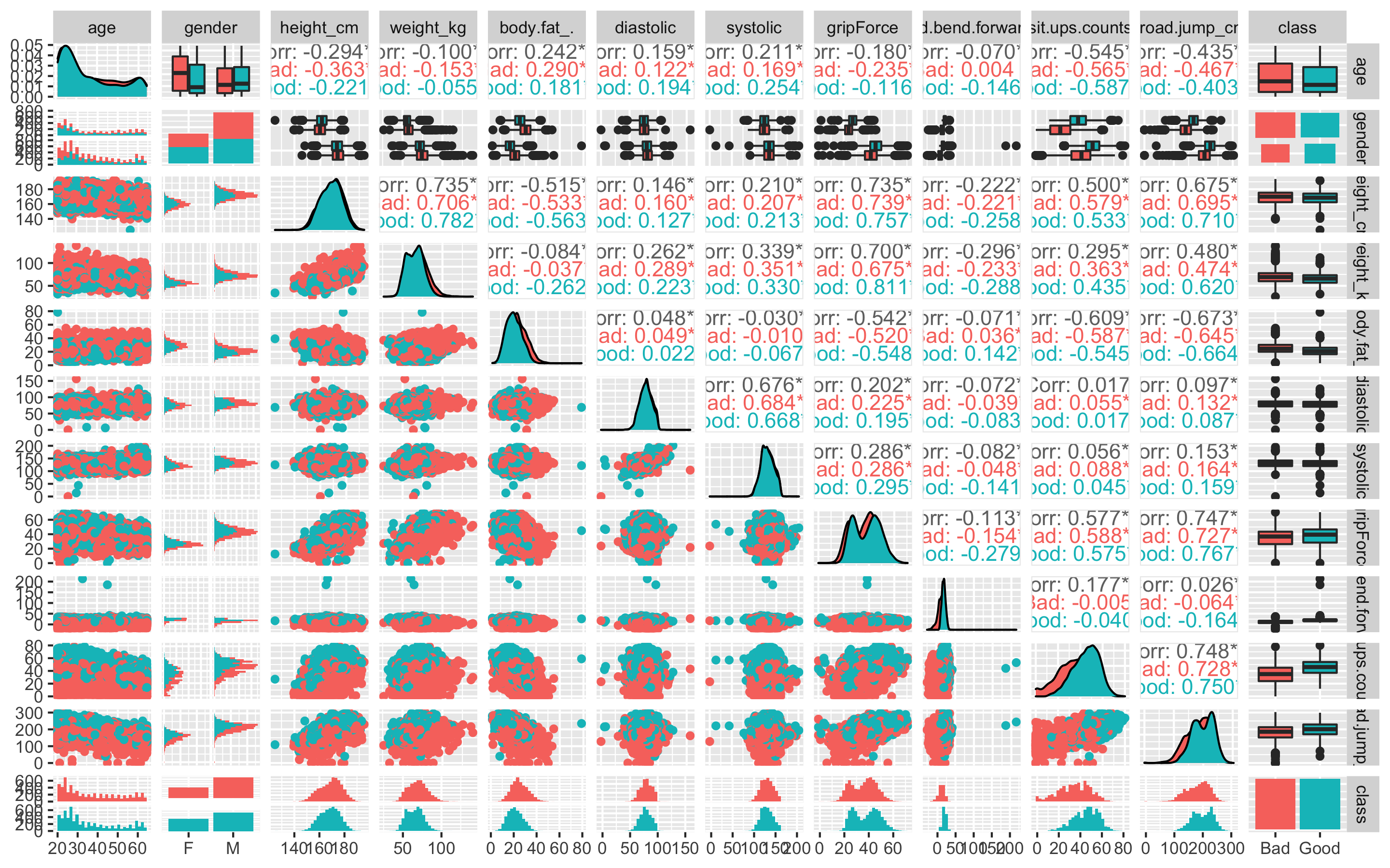
class별로 다른 색으로 그래프를 보여준다. Bad그룹이 분홍색, Good그룹이 파란색이다.
위의 탐색적 분석에서 보았듯이 sit.and.bend.forward_cm변수의 히스토그램은 왼쪽으로 쏠려있고 뾰족한 것으로 보인다.
맨 오른쪽 줄의 class열을 보면 각 수치형 변수의 boxplot을 볼 수 있는데 age를 제외한 모든 수치형 변수에 이상치가 있는 것으로 확인된다.
- ggpairs가 복잡해서 보기 힘들다면 따로 boxplot을 그려보자.
- 원래 데이터의 범위가 변수별로 차이나므로 평균이 0, 분산이 1이 되도록 스케일링 해주고, 데이터를 wide형식에서 long형식으로 바꿔준다.
> library(reshape2)
> library(caret)
> model_scale <- preProcess(df, method = c('center', 'scale'))
> scaled_df <- predict(model_scale, df)
> scaled_df_2 <- scaled_df[, -2]
> melt_df <- melt(scaled_df_2, id.vars = 'class')
> head(melt_df)
  class variable       value
1   Bad      age -0.71740533
2  Good      age -0.86418743
3   Bad      age -0.42384113
4  Good      age -0.35045008
5  Good      age -0.64401428
6 Good age -0.05688587- boxplot을 그려보자
> library(ggplot2)
> library(gridExtra)
> library(gapminder)
> library(dplyr)
> p1 <- ggplot(melt_df, aes(x = variable, y = value, fill = class)) + geom_boxplot()
> p1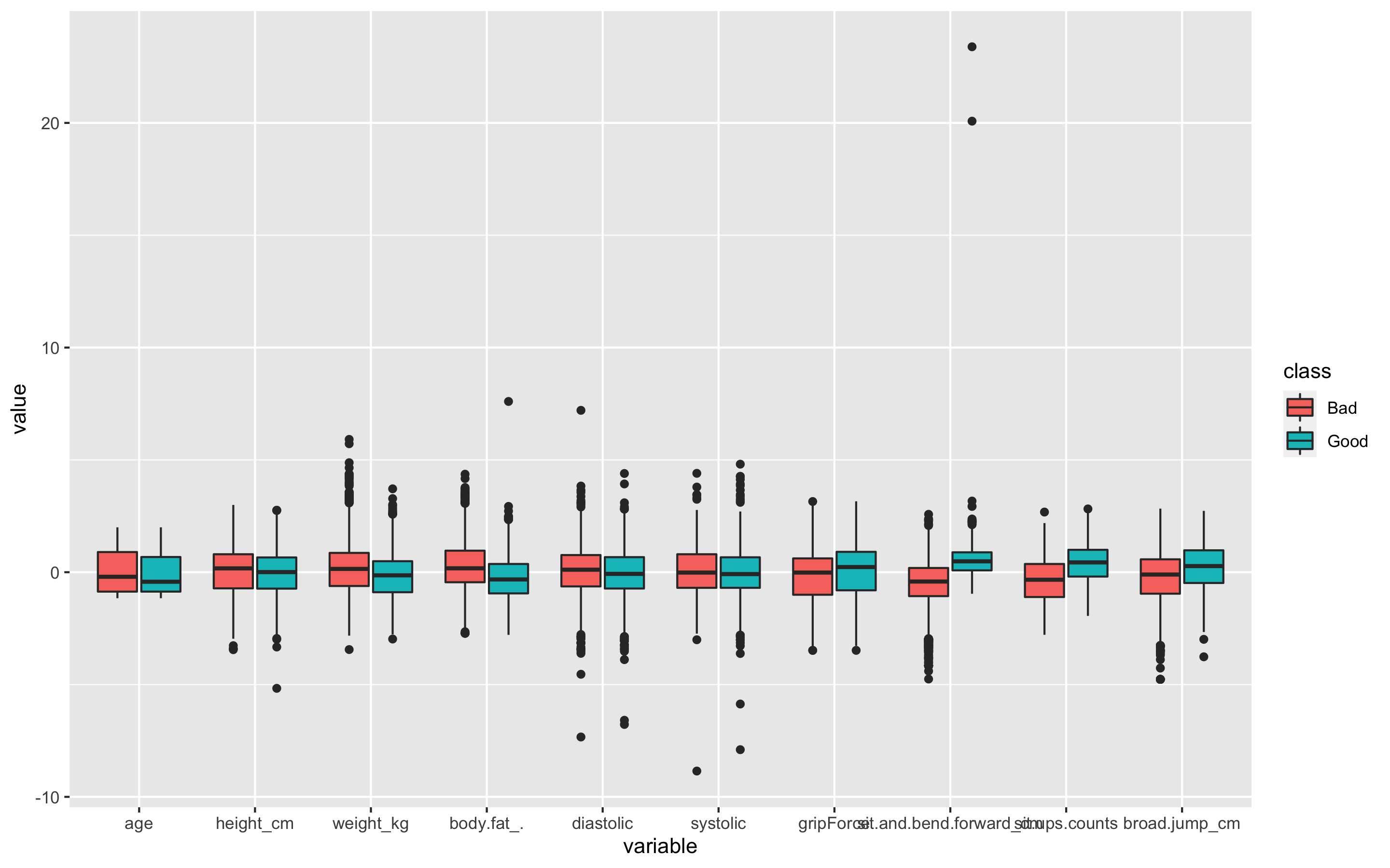
age변수를 제외한 모든 변수에 이상치가 있다. 특히 sit.and.bend.forward_cm변수에 극심한 이상치가 보인다
또한 class별 boxplot을 보았을 때, 그룹을 구별짓는 중요한 변수는 weight_kg, body.fat., sit.and.bend.forwardcm, sit.ups.counts인 것으로 추측할 수 있다.
- 사분위수 99%범위 밖의 이상치는 75% 사분위 수로 바꿔주고 1% 이내의 이상치는 25% 사분위 수로 바꿔주자.
> outHigh <- function(x){
+   x[x > quantile(x, 0.99)] <- quantile(x, 0.75)
+   x
+ }
> outLow <- function(x){
+   x[x < quantile(x, 0.01)] <- quantile(x, 0.25)
+   x
+ }
> str(df)
'data.frame':	13393 obs. of  12 variables:
 $ age                    : num  27 25 31 32 28 36 42 33 54 28 ...
 $ gender                 : Factor w/ 2 levels "F","M": 2 2 2 2 2 1 1 2 2 2 ...
 $ height_cm              : num  172 165 180 174 174 ...
 $ weight_kg              : num  75.2 55.8 78 71.1 67.7 ...
 $ body.fat_.             : num  21.3 15.7 20.1 18.4 17.1 22 32.2 36.9 27.6 14.4 ...
 $ diastolic              : num  80 77 92 76 70 64 72 84 85 81 ...
 $ systolic               : num  130 126 152 147 127 119 135 137 165 156 ...
 $ gripForce              : num  54.9 36.4 44.8 41.4 43.5 23.8 22.7 45.9 40.4 57.9 ...
 $ sit.and.bend.forward_cm: num  18.4 16.3 12 15.2 27.1 21 0.8 12.3 18.6 12.1 ...
 $ sit.ups.counts         : num  60 53 49 53 45 27 18 42 34 55 ...
 $ broad.jump_cm          : num  217 229 181 219 217 153 146 234 148 213 ...
 $ class                  : Factor w/ 2 levels "Bad","Good": 1 2 1 2 2 2 1 2 1 2 ...
> df_2 <- data.frame(lapply(df[, -c(2, 12)], outHigh))
> df_2 <- data.frame(lapply(df_2, outLow))
> df_2$gender <- df$gender
> df_2$class <- df$class
> str(df_2)
'data.frame':	13393 obs. of  12 variables:
 $ age                    : num  27 25 31 32 28 36 42 33 54 28 ...
 $ height_cm              : num  172 165 180 174 174 ...
 $ weight_kg              : num  75.2 55.8 78 71.1 67.7 ...
 $ body.fat_.             : num  21.3 15.7 20.1 18.4 17.1 22 32.2 36.9 27.6 14.4 ...
 $ diastolic              : num  80 77 92 76 70 64 72 84 85 81 ...
 $ systolic               : num  130 126 152 147 127 119 135 137 141 156 ...
 $ gripForce              : num  54.9 36.4 44.8 41.4 43.5 23.8 22.7 45.9 40.4 57.9 ...
 $ sit.and.bend.forward_cm: num  18.4 16.3 12 15.2 27.1 21 0.8 12.3 18.6 12.1 ...
 $ sit.ups.counts         : num  60 53 49 53 45 27 18 42 34 55 ...
 $ broad.jump_cm          : num  217 229 181 219 217 153 146 234 148 213 ...
 $ gender                 : Factor w/ 2 levels "F","M": 2 2 2 2 2 1 1 2 2 2 ...
$ class : Factor w/ 2 levels "Bad","Good": 1 2 1 2 2 2 1 2 1 2 ...- 이상치 변경 후의 boxplot을 그려보자
> library(reshape2)
> scale <- preProcess(df_2, method = c('center', 'scale'))
> scaled <- predict(scale, df_2)
> scaled_2 <- scaled[, -11]
> melt <- melt(scaled_2, id.vars = 'class')
> head(melt)
  class variable       value
1   Bad      age -0.71740533
2  Good      age -0.86418743
3   Bad      age -0.42384113
4  Good      age -0.35045008
5  Good      age -0.64401428
6  Good      age -0.05688587
> p2 <- ggplot(melt, aes(x = variable, y = value, fill = class)) + geom_boxplot()
> p2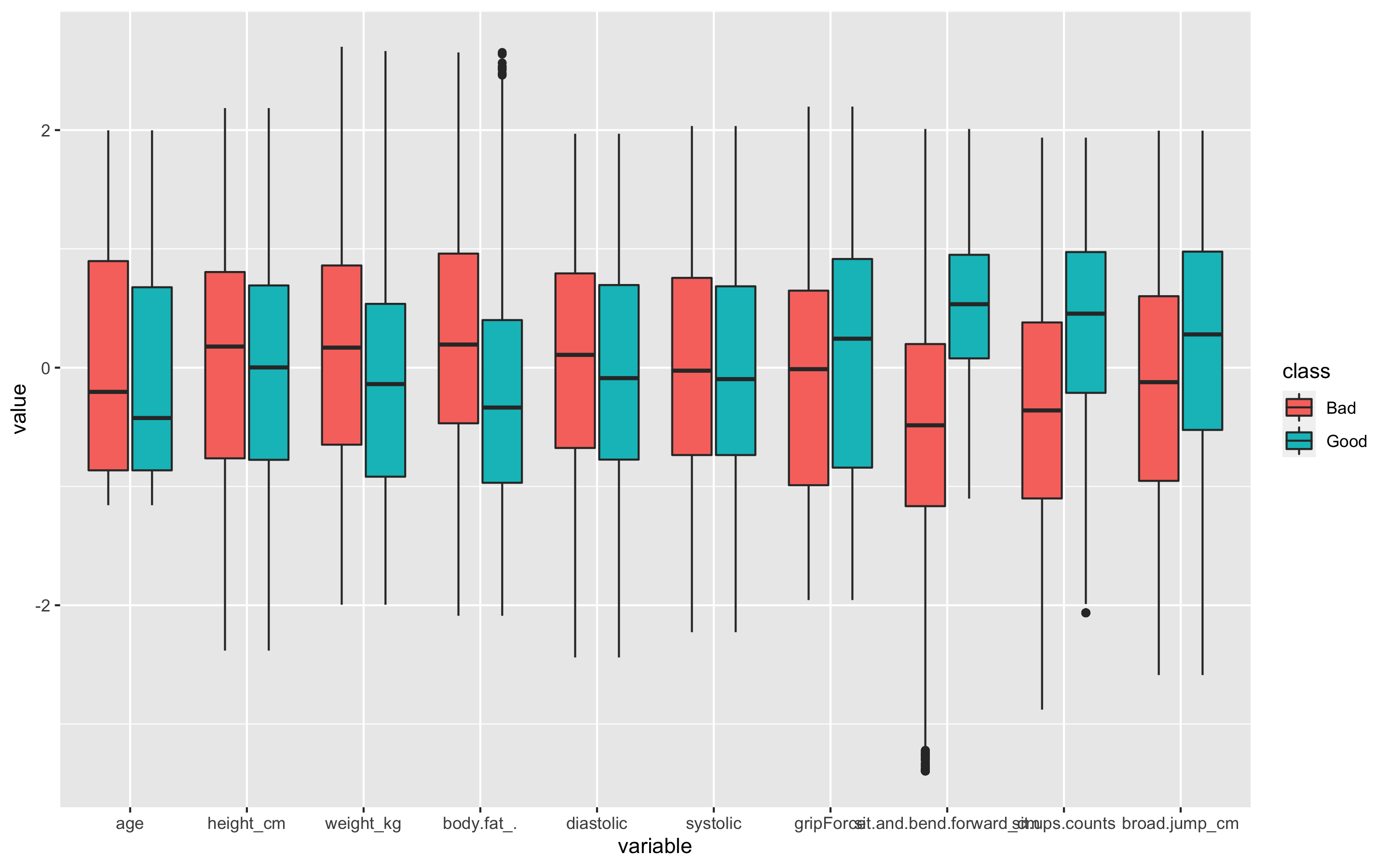
이상치는 잘 교체 된 것으로 보인다. 왜 이상치를 교체했는데도 이상치를 나타내는 점 표시가 보이냐면, 현실감 있는 데이터를 위해 양 극단의 1%의 이상치만 각각 75%, 25% 사분위수로 바꾸었기 때문이다.
- 이제 변수들의 상관관계를 확인해보자.
> df_numeric <- df_2[, -c(11, 12)]
> cor_df <- cor(df_numeric)
> cor_df
                                age  height_cm  weight_kg  body.fat_.   diastolic    systolic  gripForce
age                      1.00000000 -0.2790184 -0.0982222  0.23982512  0.15803437  0.20639817 -0.1750775
height_cm               -0.27901842  1.0000000  0.7309323 -0.51109345  0.15358942  0.22073312  0.7361757
weight_kg               -0.09822220  0.7309323  1.0000000 -0.14473537  0.26016410  0.33867687  0.7081205
body.fat_.               0.23982512 -0.5110934 -0.1447354  1.00000000  0.04155855 -0.03985372 -0.5438902
diastolic                0.15803437  0.1535894  0.2601641  0.04155855  1.00000000  0.66720616  0.2086490
systolic                 0.20639817  0.2207331  0.3386769 -0.03985372  0.66720616  1.00000000  0.2896301
gripForce               -0.17507749  0.7361757  0.7081205 -0.54389020  0.20864904  0.28963005  1.0000000
sit.and.bend.forward_cm -0.07730045 -0.2271073 -0.2976432 -0.05654621 -0.08410296 -0.09373600 -0.1383028
sit.ups.counts          -0.53851721  0.4897545  0.3158374 -0.58423814  0.01768403  0.05895636  0.5646792
broad.jump_cm           -0.42008591  0.6747026  0.5121865 -0.66090570  0.10146179  0.15957500  0.7507989
                        sit.and.bend.forward_cm sit.ups.counts broad.jump_cm
age                                -0.077300447    -0.53851721  -0.420085910
height_cm                          -0.227107295     0.48975445   0.674702577
weight_kg                          -0.297643170     0.31583738   0.512186507
body.fat_.                         -0.056546209    -0.58423814  -0.660905700
diastolic                          -0.084102956     0.01768403   0.101461794
systolic                           -0.093736000     0.05895636   0.159575001
gripForce                          -0.138302779     0.56467917   0.750798929
sit.and.bend.forward_cm             1.000000000     0.16741323   0.001790899
sit.ups.counts                      0.167413229     1.00000000   0.726531018
broad.jump_cm                       0.001790899     0.72653102   1.000000000
> library(PerformanceAnalytics)
> chart.Correlation(df_numeric, histogram = TRUE, pch = 19, method = 'pearson')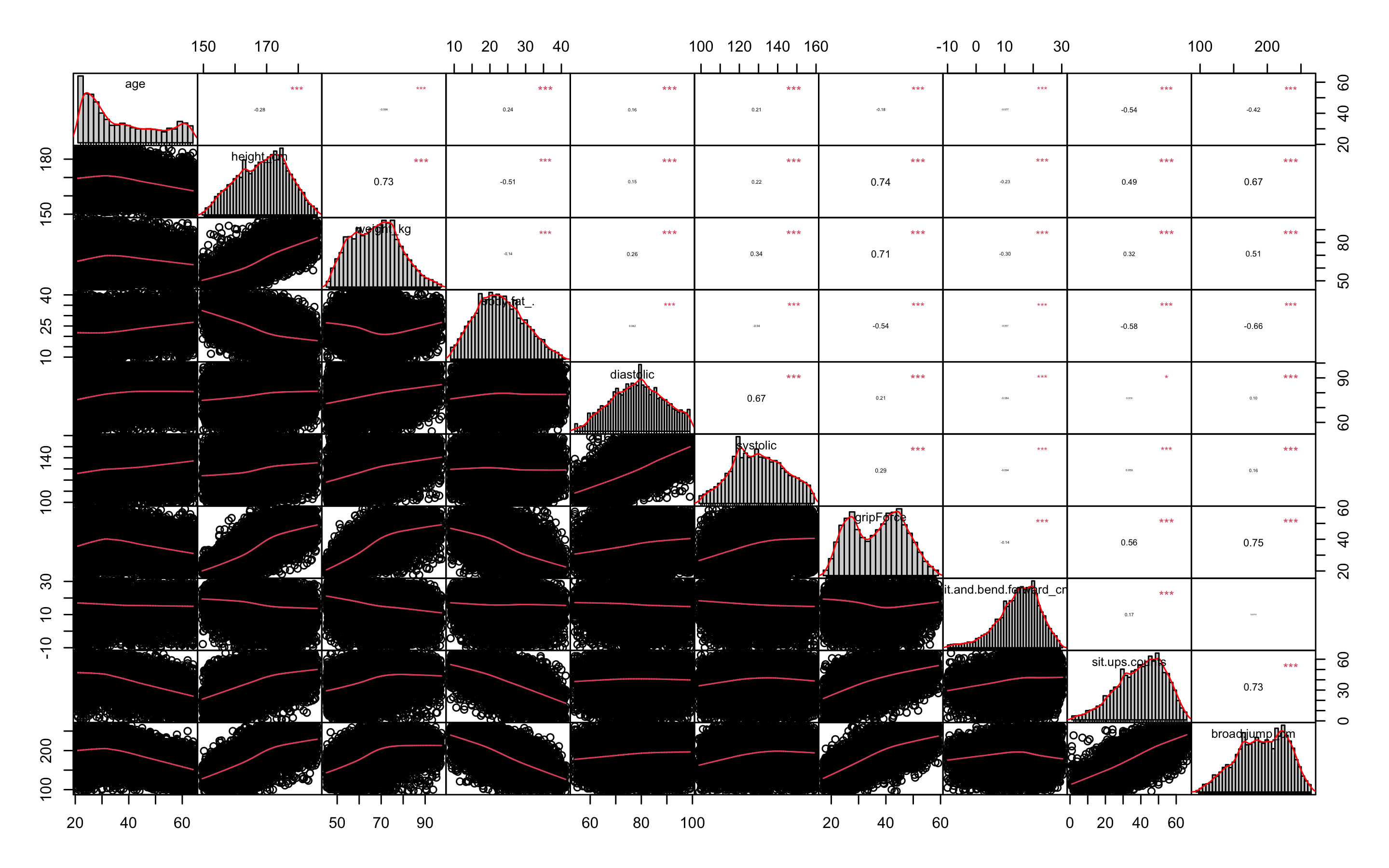
상관관계가 0.8이상인 변수가 없으므로 따로 변수를 제거하지는 않겠다.
- 분산이 0에 가까운 변수도 제거한다.
'변수를 선택하는 기법 중 가장 단순한 방법은 변숫값의 분산을 보는 것이다. 예를 들어, 데이터 1000개가 있는데 이 중 990개는 변수 A의 값이 0, 10개에서 변수 A의 값이 1이라고 하자. 그러면 변수 A는 서로 다른 관찰을 구별하는 데 별 소용이 없다. 따라서 데이터 모델링에서도 그리 유용하지 않다. 이런 변수는 분산이 0에 가까우므로 분석 전에 제거해준다.
> nearZeroVar(df_numeric, saveMetrics = TRUE)
                        freqRatio percentUnique zeroVar   nzv
age                      1.221800     0.3285298   FALSE FALSE
height_cm                1.052326     2.7253043   FALSE FALSE
weight_kg                1.042424     9.2511013   FALSE FALSE
body.fat_.               1.005376     3.1135668   FALSE FALSE
diastolic                1.390041     0.3583962   FALSE FALSE
systolic                 1.500000     0.4554618   FALSE FALSE
gripForce                1.073034     3.1882327   FALSE FALSE
sit.and.bend.forward_cm  1.040000     3.1285000   FALSE FALSE
sit.ups.counts           1.171875     0.5077279   FALSE FALSE
broad.jump_cm            1.061224     1.2917196   FALSE FALSE
분산이 0에 가까운 변수는 없다!(분산이 0에 가까운 변수는 위 출력의 nzv부분이 TRUE로 나온다)
- Boruta패키지를 사용해 변수 선택을 해보자
> library(Boruta)
> set.seed(123)
> feature.selection <- Boruta(class ~., data = df_2, doTrace = 1)
> table(feature.selection$finalDecision)

Tentative Confirmed  Rejected
        0        11         0
거절되거나 거절하기 긴가민가한(tentative)변수는 없는 것으로 판명되었다.
- 데이터를 train데이터와 test데이터로 분리하자.
> library(caret)
> idx <- createDataPartition(df_2$class, p = 0.7)
> train <- df_2[idx$Resample1, ]
> test <- df_2[-idx$Resample1, ]
> table(train$class)

 Bad Good
4689 4687
결과변수 class의 Bad그룹과 Good그룹의 데이터 개수가 거의 유사하므로 업샘플링이나 SMOTE는 진행하지 않는다.
- train데이터와 test데이터의 예측변수가 더미변수여야만 진행되는 분석을 위해 미리 더미변수화 해주자.
> dummies <- dummyVars(class ~., data = train)
> dummies
Dummy Variable Object

Formula: class ~ .
12 variables, 2 factors
Variables and levels will be separated by '.'
A less than full rank encoding is used
> train_dummy <- as.data.frame(predict(dummies, newdata = train))
Warning message:
In model.frame.default(Terms, newdata, na.action = na.action, xlev = object$lvls) :
  variable 'class' is not a factor
> str(train_dummy)
'data.frame':	9376 obs. of  12 variables:
 $ age                    : num  25 32 36 33 28 42 27 22 24 45 ...
 $ height_cm              : num  165 174 165 175 185 ...
 $ weight_kg              : num  55.8 71.1 55.4 77.2 84.6 65.4 53.9 67.9 84.4 63.1 ...
 $ body.fat_.             : num  15.7 18.4 22 36.9 14.4 19.3 35.5 11.3 20.4 30.9 ...
 $ diastolic              : num  77 76 64 84 81 63 69 71 80 93 ...
 $ systolic               : num  126 147 119 137 156 110 116 103 120 144 ...
 $ gripForce              : num  36.4 41.4 23.8 45.9 57.9 43.5 23.1 52.5 48.9 34.1 ...
 $ sit.and.bend.forward_cm: num  16.3 15.2 21 12.3 12.1 16 13.1 19.2 7.2 19 ...
 $ sit.ups.counts         : num  53 53 27 42 55 50 28 55 54 30 ...
 $ broad.jump_cm          : num  229 219 153 234 213 211 144 232 213 155 ...
 $ gender.F               : num  0 0 1 0 0 0 1 0 0 1 ...
 $ gender.M               : num  1 1 0 1 1 1 0 1 1 0 ...
> train_dummy$class <- train$class

> dummies2 <- dummyVars(class ~., data = test)
> test_dummy <- as.data.frame(predict(dummies2, newdata = test))
Warning message:
In model.frame.default(Terms, newdata, na.action = na.action, xlev = object$lvls) :
  variable 'class' is not a factor
> str(test_dummy)
'data.frame':	4017 obs. of  12 variables:
 $ age                    : num  27 31 28 42 54 57 26 25 49 31 ...
 $ height_cm              : num  172 180 174 164 167 ...
 $ weight_kg              : num  75.2 78 67.7 63.7 67.5 ...
 $ body.fat_.             : num  21.3 20.1 17.1 32.2 27.6 20.9 21 15.7 27.6 23 ...
 $ diastolic              : num  80 92 70 72 85 69 63 80 77 90 ...
 $ systolic               : num  130 152 127 135 141 106 129 127 144 148 ...
 $ gripForce              : num  54.9 44.8 43.5 22.7 40.4 21.5 41.3 36.4 23.8 51.2 ...
 $ sit.and.bend.forward_cm: num  18.4 12 27.1 0.8 18.6 30 15.1 26.4 21.3 18.4 ...
 $ sit.ups.counts         : num  60 49 45 18 34 30 53 38 39 62 ...
 $ broad.jump_cm          : num  217 181 217 146 148 162 225 246 154 208 ...
 $ gender.F               : num  0 0 0 1 0 1 0 0 1 0 ...
 $ gender.M               : num  1 1 1 0 1 0 1 1 0 1 ...
> test_dummy$class <- test$class- 데이터 정규화가 필요한 모델링을 위해 미리 정규화 작업을 해준다.
> model_train <- preProcess(train, method = c('center', 'scale'))
> model_test <- preProcess(test, method = c('center', 'scale'))
> scaled_train <- predict(model_train, train)
> scaled_test <- predict(model_test, test)- 마찬가지로 scaled_train데이터와 scaled_test데이터도 미리 더미변수화 해준다.
> dummies3 <- dummyVars(class ~., data = scaled_train)
> scaled_train_dummy <- as.data.frame(predict(dummies3, newdata = scaled_train))
Warning message:
In model.frame.default(Terms, newdata, na.action = na.action, xlev = object$lvls) :
  variable 'class' is not a factor
> str(scaled_train_dummy)
'data.frame':	9376 obs. of  12 variables:
 $ age                    : num  -0.8656 -0.3496 -0.0547 -0.2759 -0.6445 ...
 $ height_cm              : num  -0.453 0.745 -0.403 0.796 2.07 ...
 $ weight_kg              : num  -1.035 0.337 -1.071 0.884 1.547 ...
 $ body.fat_.             : num  -1.111 -0.712 -0.179 2.026 -1.303 ...
 $ diastolic              : num  -0.185 -0.283 -1.46 0.501 0.207 ...
 $ systolic               : num  -0.308 1.186 -0.806 0.475 1.827 ...
 $ gripForce              : num  -0.054 0.441 -1.301 0.886 2.074 ...
 $ sit.and.bend.forward_cm: num  0.136 -0.012 0.767 -0.402 -0.428 ...
 $ sit.ups.counts         : num  0.977 0.977 -0.959 0.158 1.126 ...
 $ broad.jump_cm          : num  1.037 0.768 -1.01 1.172 0.606 ...
 $ gender.F               : num  0 0 1 0 0 0 1 0 0 1 ...
 $ gender.M               : num  1 1 0 1 1 1 0 1 1 0 ...
> scaled_train_dummy$class <- scaled_train$class
> dummies4 <- dummyVars(class ~., data = scaled_test)
> scaled_test_dummy <- as.data.frame(predict(dummies4, newdata = scaled_test))
Warning message:
In model.frame.default(Terms, newdata, na.action = na.action, xlev = object$lvls) :
  variable 'class' is not a factor
> str(scaled_test_dummy)
'data.frame':	4017 obs. of  12 variables:
 $ age                    : num  -0.716 -0.425 -0.643 0.374 1.246 ...
 $ height_cm              : num  0.463 1.367 0.649 -0.503 -0.218 ...
 $ weight_kg              : num  0.7186 0.9674 0.039 -0.3216 0.0209 ...
 $ body.fat_.             : num  -0.264 -0.438 -0.876 1.324 0.654 ...
 $ diastolic              : num  0.106 1.28 -0.872 -0.677 0.595 ...
 $ systolic               : num  -0.0295 1.5249 -0.2414 0.3238 0.7477 ...
 $ gripForce              : num  1.765 0.775 0.648 -1.389 0.344 ...
 $ sit.and.bend.forward_cm: num  0.404 -0.452 1.566 -1.948 0.43 ...
 $ sit.ups.counts         : num  1.478 0.673 0.38 -1.597 -0.425 ...
 $ broad.jump_cm          : num  0.697 -0.257 0.697 -1.184 -1.131 ...
 $ gender.F               : num  0 0 0 1 0 1 0 0 1 0 ...
 $ gender.M               : num  1 1 1 0 1 0 1 1 0 1 ...
> scaled_test_dummy$class <- scaled_test$class
KNN
- KNN분석을 해보자.
- KNN은 scale된 데이터와, 예측변수에 팩터형 변수가 있다면 더미변수로 바꿔줘야 한다.
- 위에서 미리 만들어둔 scaled_train_dummy데이터와 scaled_test_dummy데이터를 사용하자.
- KNN을 사용할 때는 가장 적절한 K를 선택하는 일은 매우 중요하다. K를 선택하기 위해 expand.grid()와 seq()함수를 사용해보자.
> library(class)
> library(kknn)
> library(e1071)
> library(caret)
> library(MASS)
> library(reshape2)
> library(ggplot2)
> library(kernlab)
> library(corrplot)
> grid1 <- expand.grid(.k = seq(2, 30, by = 1))
> control <- trainControl(method = 'cv')
> set.seed(123)
> knn.train <- train(class ~., data = scaled_train_dummy,
+                    method = 'knn',
+                    trControl = control,
+                    tuneGrid = grid1)
> knn.train
k-Nearest Neighbors

9376 samples
  12 predictor
   2 classes: 'Bad', 'Good'

No pre-processing
Resampling: Cross-Validated (10 fold)
Summary of sample sizes: 8439, 8438, 8438, 8438, 8438, 8439, ...
Resampling results across tuning parameters:

  k   Accuracy   Kappa
   2  0.7657843  0.5315784
   3  0.8051407  0.6102936
   4  0.8008769  0.6017611
   5  0.8118617  0.6237357
   6  0.8111131  0.6222392
.
.
.
  20  0.8247644  0.6495440
  21  0.8238058  0.6476274
  22  0.8225261  0.6450678
  23  0.8219925  0.6440002
  24  0.8209269  0.6418696
  25  0.8215665  0.6431486
  26  0.8217795  0.6435736
  27  0.8211393  0.6422945
  28  0.8199654  0.6399472
  29  0.8209260  0.6418680
  30  0.8204990  0.6410142

Accuracy was used to select the optimal model using the
 largest value.
The final value used for the model was k = 20.
k매개변수 값으로 20이 나왔다. k값을 20으로 사용할 때의 카파통계량은 0.6495이다.
- 🍎Kappa 통계량
카파 통계량은 흔히 두 평가자가 관찰값을 분류할 때 서로 동의하는 정도를 재는 척도로 쓰인다. 카파 통계량은 정확도 점수를 조정함으로써 당면 문제에 관한 통찰력을 제공한다. 이때 조정은 평가자가 모든 분류를 정확히 맞췄을 경우에서 단지 우연을 맞췄을 경우를 빼는 방식으로 이뤄진다. 카파통계량의 값이 높을수록 평가자들의 성능이 높은 것이고, 가능한 최댓값은 1이다. 알트만(Altman, 1911)은 이 통계량의 값을 해석하기 위한 경험적 기법을 아래의 표와 같이 제공한다.
| K값 | 동의의 강도 |
|---|---|
| < 0.2 | Poor(약함) |
| 0.21 ~ 0.4 | Fair(약간 동의) |
| 0.41 ~ 0.6 | Moderate(어느 정도 동의) |
| 0.61 ~ 0.8 | Good(상당히 동의) |
| 0.81 ~ 1 | Very Good(매우 동의) |
- 다시 KNN으로 돌아가 분석을 해보자.
> knn.test <- knn(scaled_train_dummy[, -13], scaled_test_dummy[, -13], scaled_train_dummy[, 13], k = 20)
> confusionMatrix(knn.test, scaled_test_dummy$class, positive = 'Good')
Confusion Matrix and Statistics

          Reference
Prediction  Bad Good
      Bad  1478  163
      Good  531 1845

               Accuracy : 0.8272
                 95% CI : (0.8152, 0.8388)
    No Information Rate : 0.5001
    P-Value [Acc > NIR] : < 2.2e-16

                  Kappa : 0.6545

 Mcnemar's Test P-Value : < 2.2e-16

            Sensitivity : 0.9188
            Specificity : 0.7357
         Pos Pred Value : 0.7765
         Neg Pred Value : 0.9007
             Prevalence : 0.4999
         Detection Rate : 0.4593
   Detection Prevalence : 0.5915
      Balanced Accuracy : 0.8273

       'Positive' Class : Good
정확도는 약 82.7%, 카파통계량은 0.6545가 나왔다.
- 성능을 더 올리기 위해 커널을 입력해보자.
> kknn.train <- train.kknn(class ~., data = scaled_train_dummy, kmax = 30, distance = 2,
+                          kernel = c('rectangular', 'triangular', 'epanechnikov'))
> plot(kknn.train)
distance = 2는 절댓값합 거리를 사용함을 의미하고 1로 설정하면 유클리드 거리를 의미한다.
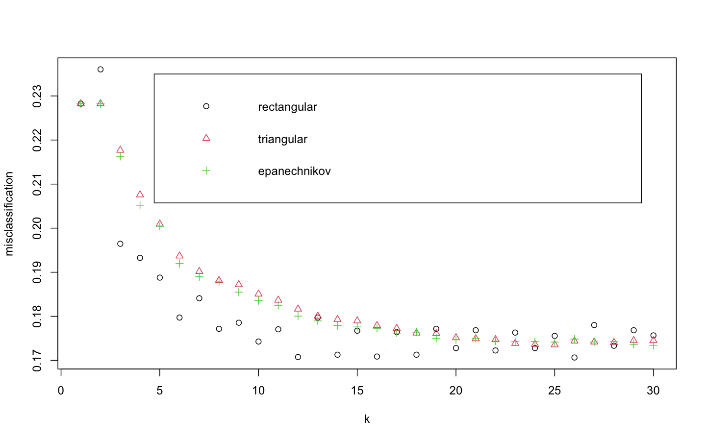
위의 plot은 k값을 x축, 각 커널에 의해 잘못 분류된 관찰값의 비율을 y축에 표시하고 있다. 얼핏보았을 때 k가 26일 때 rectangular커널을 사용했을 때 가장 오류가 낮은 것으로 보인다.
- 더 정확히 살펴보자.
> kknn.train

Call:
train.kknn(formula = class ~ ., data = scaled_train_dummy, kmax = 30,     distance = 2, kernel = c("rectangular", "triangular", "epanechnikov"))

Type of response variable: nominal
Minimal misclassification: 0.1706485
Best kernel: rectangular
Best k: 26- predict()함수를 사용해 예측해보자.
> kknn.pred <- predict(kknn.train, newdata = scaled_test_dummy)
> confusionMatrix(kknn.pred, scaled_test_dummy$class, positive = 'Good')
Confusion Matrix and Statistics

          Reference
Prediction  Bad Good
      Bad  1476  164
      Good  533 1844

               Accuracy : 0.8265
                 95% CI : (0.8144, 0.8381)
    No Information Rate : 0.5001
    P-Value [Acc > NIR] : < 2.2e-16

                  Kappa : 0.653

 Mcnemar's Test P-Value : < 2.2e-16

            Sensitivity : 0.9183
            Specificity : 0.7347
         Pos Pred Value : 0.7758
         Neg Pred Value : 0.9000
             Prevalence : 0.4999
         Detection Rate : 0.4590
   Detection Prevalence : 0.5917
      Balanced Accuracy : 0.8265

       'Positive' Class : Good
커널을 사용하지 않았을 때(정확도 82.7%, 카파통계량 0.6545)보다 커널을 사용했을 때(정확도 82.65%, 카파통계량 0.653) 오히려 성능이 미세하게 떨어졌다.
SVM
- SVM분석을 해보자.
- SVM은 scale된 데이터를 사용해야 하므로 scaled_train, scaled_test데이터를 사용하겠다.
- e1071패키지의 tune.svm()함수를 이용해 튜닝 파라미터 및 커널함수를 선택하자.
> linear.tune <- tune.svm(class ~., data = scaled_train,
+                         kernel = 'linear',
+                         cost = c(0.001, 0.01, 0.1, 0.5, 1, 2, 5, 10))
> summary(linear.tune)

Parameter tuning of ‘svm’:

- sampling method: 10-fold cross validation

- best parameters:
 cost
  0.1

- best performance: 0.1789719

- Detailed performance results:
   cost     error dispersion
1 1e-03 0.1913448 0.01661437
2 1e-02 0.1818523 0.02012465
3 1e-01 0.1789719 0.01858989
4 5e-01 0.1790785 0.01819574
5 1e+00 0.1791853 0.01848974
6 2e+00 0.1791854 0.01893003
7 5e+00 0.1791855 0.01883092
8 1e+01 0.1791854 0.01864774
최적의 cost함수는 0.1로 나왔다.
- predict()함수로 test데이터 예측을 실행해보자.
> best.linear <- linear.tune$best.model
> tune.test <- predict(best.linear, newdata = scaled_test)
> confusionMatrix(tune.test, scaled_test$class, positive = 'Good')
Confusion Matrix and Statistics

          Reference
Prediction  Bad Good
      Bad  1607  279
      Good  402 1729

               Accuracy : 0.8305
                 95% CI : (0.8185, 0.842)
    No Information Rate : 0.5001
    P-Value [Acc > NIR] : < 2.2e-16

                  Kappa : 0.6609

 Mcnemar's Test P-Value : 2.939e-06

            Sensitivity : 0.8611
            Specificity : 0.7999
         Pos Pred Value : 0.8114
         Neg Pred Value : 0.8521
             Prevalence : 0.4999
         Detection Rate : 0.4304
   Detection Prevalence : 0.5305
      Balanced Accuracy : 0.8305

       'Positive' Class : Good
정확도는 약 83.05%, 카파통계량은 0.6609로 KNN모델에서 보였던 성능보다 좋은 성능을 보인다.
- polynomial커널함수를 사용해 degree와 커널계수를 조정해보자. degree는 3, 4, 5의 값을 주고 coef0은 0.1부터 4까지의 숫자를 준다.
> set.seed(123)
> poly.tune <- tune.svm(class ~., data = scaled_train,
+                       kernel = 'polynomial', degree = c(3, 4, 5),
+                       coef0 = c(0.1, 0.5, 1, 2, 3, 4))
Warning messages:
1: In doTryCatch(return(expr), name, parentenv, handler) :
  restarting interrupted promise evaluation
2: In .rs.normalizePath(filePath) : path[1]="": No such file or directory
3: In .rs.normalizePath(filePath) : path[1]="": No such file or directory
> summary(poly.tune)

Parameter tuning of ‘svm’:

- sampling method: 10-fold cross validation

- best parameters:
 degree coef0
      4     4

- best performance: 0.1388665

- Detailed performance results:
   degree coef0     error  dispersion
1       3   0.1 0.1550778 0.007102034
2       4   0.1 0.1509189 0.010600932
3       5   0.1 0.1594524 0.010046621
4       3   0.5 0.1452656 0.006785186
5       4   0.5 0.1445196 0.008461263
6       5   0.5 0.1460129 0.007702409
7       3   1.0 0.1443066 0.007682120
8       4   1.0 0.1425995 0.007504729
9       5   1.0 0.1429196 0.006686115
10      3   2.0 0.1409997 0.006488216
11      4   2.0 0.1405736 0.007511930
12      5   2.0 0.1451588 0.004965223
13      3   3.0 0.1407868 0.007969374
14      4   3.0 0.1393995 0.006368466
15      5   3.0 0.1475052 0.006987889
16      3   4.0 0.1414268 0.007501050
17      4   4.0 0.1388665 0.007414464
18      5   4.0 0.1468653 0.006521403
_최적의 degree는 4고, coef0는 4이다.
- predict()함수로 test데이터를 사용해 예측을 해보자.
> best.poly <- poly.tune$best.model
> poly.test <- predict(best.poly, newdata = scaled_test)
> confusionMatrix(poly.test, scaled_test$class, positive = 'Good')
Confusion Matrix and Statistics

          Reference
Prediction  Bad Good
      Bad  1658  187
      Good  351 1821

               Accuracy : 0.8661
                 95% CI : (0.8551, 0.8765)
    No Information Rate : 0.5001
    P-Value [Acc > NIR] : < 2.2e-16

                  Kappa : 0.7321

 Mcnemar's Test P-Value : 2.104e-12

            Sensitivity : 0.9069
            Specificity : 0.8253
         Pos Pred Value : 0.8384
         Neg Pred Value : 0.8986
             Prevalence : 0.4999
         Detection Rate : 0.4533
   Detection Prevalence : 0.5407
      Balanced Accuracy : 0.8661

       'Positive' Class : Good
정확도는 약 86.61%, 카파통계량은 0.7321로 선형 SVM모델보다 더 좋은 성능을 보인다.
- 다음으로 커널 함수로 시그모이드를 설정해보자. 매개변수인 gamma와 coef0이 최적의 값이 되도록 계산해보자.
> set.seed(123)
> sigmoid.tune <- tune.svm(class ~., data = scaled_train,
+                          kernel = 'sigmoid',
+                          gamma = c(0.1, 0.5, 1, 2, 3, 4),
+                          coef0 = c(0.1, 0.5, 1, 2, 3, 4))
> summary(sigmoid.tune)

Parameter tuning of ‘svm’:

- sampling method: 10-fold cross validation

- best parameters:
 gamma coef0
   0.1   0.1

- best performance: 0.3521784

- Detailed performance results:
   gamma coef0     error dispersion
1    0.1   0.1 0.3521784 0.01419968
2    0.5   0.1 0.4474222 0.02119956
3    1.0   0.1 0.4603266 0.02138924
4    2.0   0.1 0.4638463 0.02132723
5    3.0   0.1 0.4656602 0.02326069
.
.
.
30   4.0   3.0 0.4409171 0.02253223
31   0.1   4.0 0.3808680 0.01469343
32   0.5   4.0 0.4458245 0.01794936
33   1.0   4.0 0.4310984 0.00752699
34   2.0   4.0 0.4035826 0.03069074
35   3.0   4.0 0.4393199 0.02047452
36   4.0   4.0 0.4372932 0.01987919
최적의 gamma값은 0.1, coef0값은 0.1로 나왔다.
- predict()함수로 test데이터를 사용해 예측을 해보자.
> best.sigmoid <- sigmoid.tune$best.model
> sigmoid.test <- predict(best.sigmoid, newdata = scaled_test)
> confusionMatrix(sigmoid.test, scaled_test$class, positive = 'Good')
Confusion Matrix and Statistics

          Reference
Prediction  Bad Good
      Bad  1321  695
      Good  688 1313

               Accuracy : 0.6557
                 95% CI : (0.6408, 0.6704)
    No Information Rate : 0.5001
    P-Value [Acc > NIR] : <2e-16

                  Kappa : 0.3114

 Mcnemar's Test P-Value : 0.8718

            Sensitivity : 0.6539
            Specificity : 0.6575
         Pos Pred Value : 0.6562
         Neg Pred Value : 0.6553
             Prevalence : 0.4999
         Detection Rate : 0.3269
   Detection Prevalence : 0.4981
      Balanced Accuracy : 0.6557

       'Positive' Class : Good
정확도는 약 65.57%, 카파통계량은 0.3114로 polynomial커널함수를 사용한 SVM모델보다 성능이 훨씬 떨어졌다.
- 마지막으로 커널 함수로 radial을 설정해 최적의 gamma값을 계산해보자.
> rbf.tune <- tune.svm(class ~., data = scaled_train,
+                      kernel = 'radial',
+                      gamma = c(0.1, 0.5, 1, 2, 3, 4))
> summary(rbf.tune)

Parameter tuning of ‘svm’:

- sampling method: 10-fold cross validation

- best parameters:
 gamma
   0.1

- best performance: 0.1466525

- Detailed performance results:
  gamma     error  dispersion
1   0.1 0.1466525 0.006558098
2   0.5 0.1499569 0.008083620
3   1.0 0.1625426 0.008591551
4   2.0 0.2031797 0.010492578
5   3.0 0.2522444 0.016097913
6   4.0 0.2881874 0.016905457
최적의 gamma값은 0.1로 나왔다.
- predict()함수로 test데이터를 사용해 예측을 해보자.
> best.rbf <- rbf.tune$best.model
> rbf.test <- predict(best.rbf, newdata = scaled_test)
> confusionMatrix(rbf.test, scaled_test$class, positive = 'Good')
Confusion Matrix and Statistics

          Reference
Prediction  Bad Good
      Bad  1647  225
      Good  362 1783

               Accuracy : 0.8539
                 95% CI : (0.8426, 0.8647)
    No Information Rate : 0.5001
    P-Value [Acc > NIR] : < 2.2e-16

                  Kappa : 0.7077

 Mcnemar's Test P-Value : 1.985e-08

            Sensitivity : 0.8879
            Specificity : 0.8198
         Pos Pred Value : 0.8312
         Neg Pred Value : 0.8798
             Prevalence : 0.4999
         Detection Rate : 0.4439
   Detection Prevalence : 0.5340
      Balanced Accuracy : 0.8539

       'Positive' Class : Good
정확도는 약 85.39%, 카파통계량은 0.7077이다.
SVM모델 중 polynomial커널함수를 사용한 모델이 정확도 약 86.61%, 카파통계량0.7321로 가장 좋은 성능을 보인다.
랜덤포레스트
- 다음으로 랜덤포레스트 모델을 만들어 보자.
> library(rpart)
> library(partykit)
> library(MASS)
> library(genridge)
> library(randomForest)
> library(xgboost)
> library(caret)
> library(Boruta)
> rfmodel <- randomForest(class ~., data = train)
> rfmodel

Call:
 randomForest(formula = class ~ ., data = train)
               Type of random forest: classification
                     Number of trees: 500
No. of variables tried at each split: 3

        OOB estimate of  error rate: 13.34%
Confusion matrix:
      Bad Good class.error
Bad  3918  771   0.1644274
Good  480 4207   0.1024109
수행 결과 OOB(out of bag)오차율은 13.34%가 나왔다.
- 개선을 위해 최적의 트리 수를 보자.
> plot(rfmodel)
> which.min(rfmodel$err.rate[, 1])
[1] 436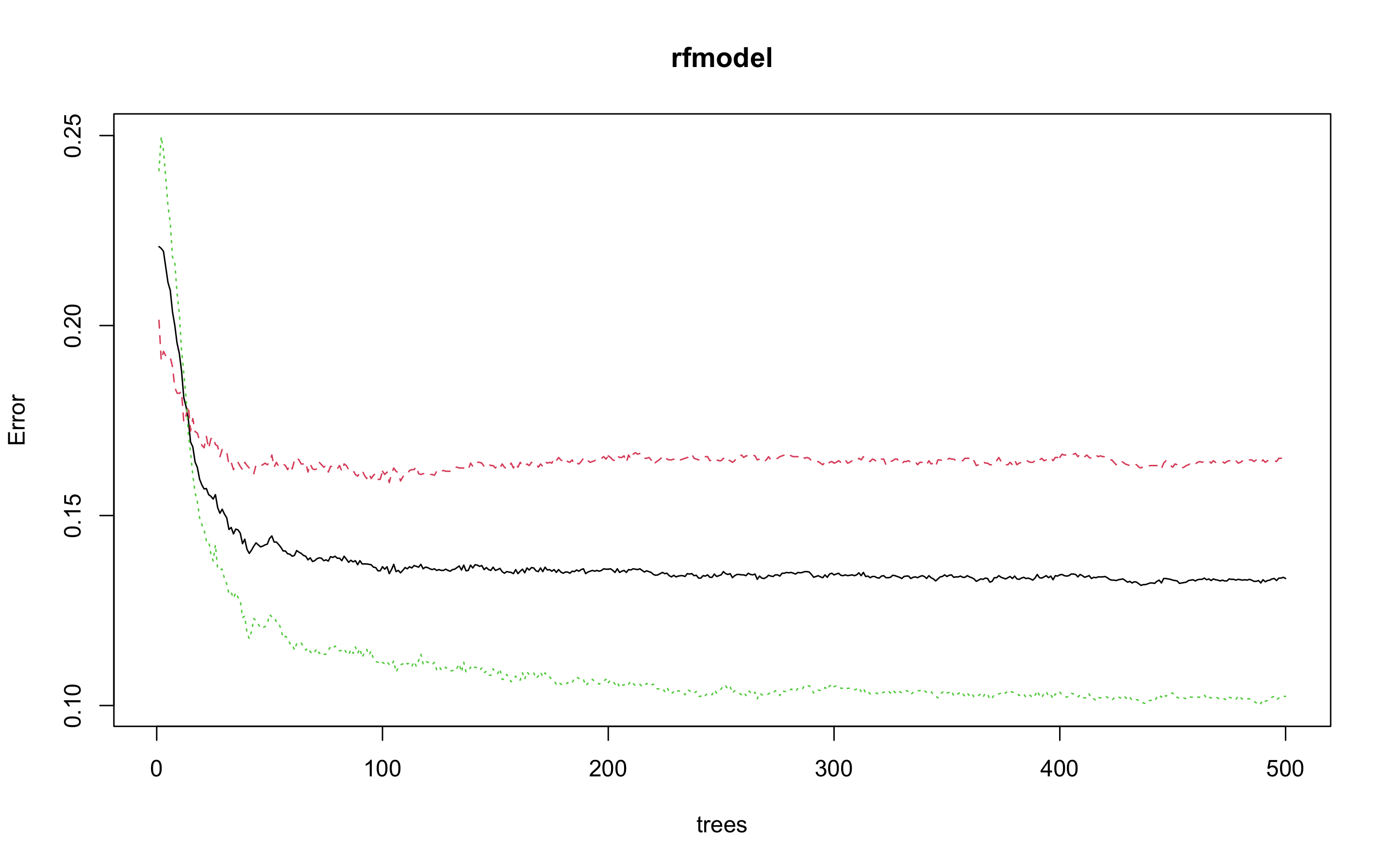
_모델 정확도를 최적화하기에 필요한 트리수가 436개라는 결과를 얻었다.
> rfmodel2 <- randomForest(class ~., data = train, ntree = 436)
> rfmodel2

Call:
 randomForest(formula = class ~ ., data = train, ntree = 436)
               Type of random forest: classification
                     Number of trees: 436
No. of variables tried at each split: 3

        OOB estimate of  error rate: 13.2%
Confusion matrix:
      Bad Good class.error
Bad  3927  762   0.1625080
Good  476 4211   0.1015575
OOB 오차율이 13.34%에서 13.2%로 아주 약간 줄었다.
- test데이터로 어떤 결과가 나오는지 보자.
> rftest <- predict(rfmodel2, newdata = test, type = 'response')
> confusionMatrix(rftest, test$class, positive = 'Good')
Confusion Matrix and Statistics

          Reference
Prediction  Bad Good
      Bad  1686  194
      Good  323 1814

               Accuracy : 0.8713
                 95% CI : (0.8605, 0.8815)
    No Information Rate : 0.5001
    P-Value [Acc > NIR] : < 2.2e-16

                  Kappa : 0.7426

 Mcnemar's Test P-Value : 1.808e-08

            Sensitivity : 0.9034
            Specificity : 0.8392
         Pos Pred Value : 0.8489
         Neg Pred Value : 0.8968
             Prevalence : 0.4999
         Detection Rate : 0.4516
   Detection Prevalence : 0.5320
      Balanced Accuracy : 0.8713

       'Positive' Class : Good
정확도 87.13%, 카파통계량 0.7426으로 SVM모델 중 polynomial커널함수를 사용한 모델(정확도 86.61%, 카파통계량0.7321)보다 약간 더 좋은 성능을 보인다.
- 변수 중요도를 보자.
varImpPlot(rfmodel2)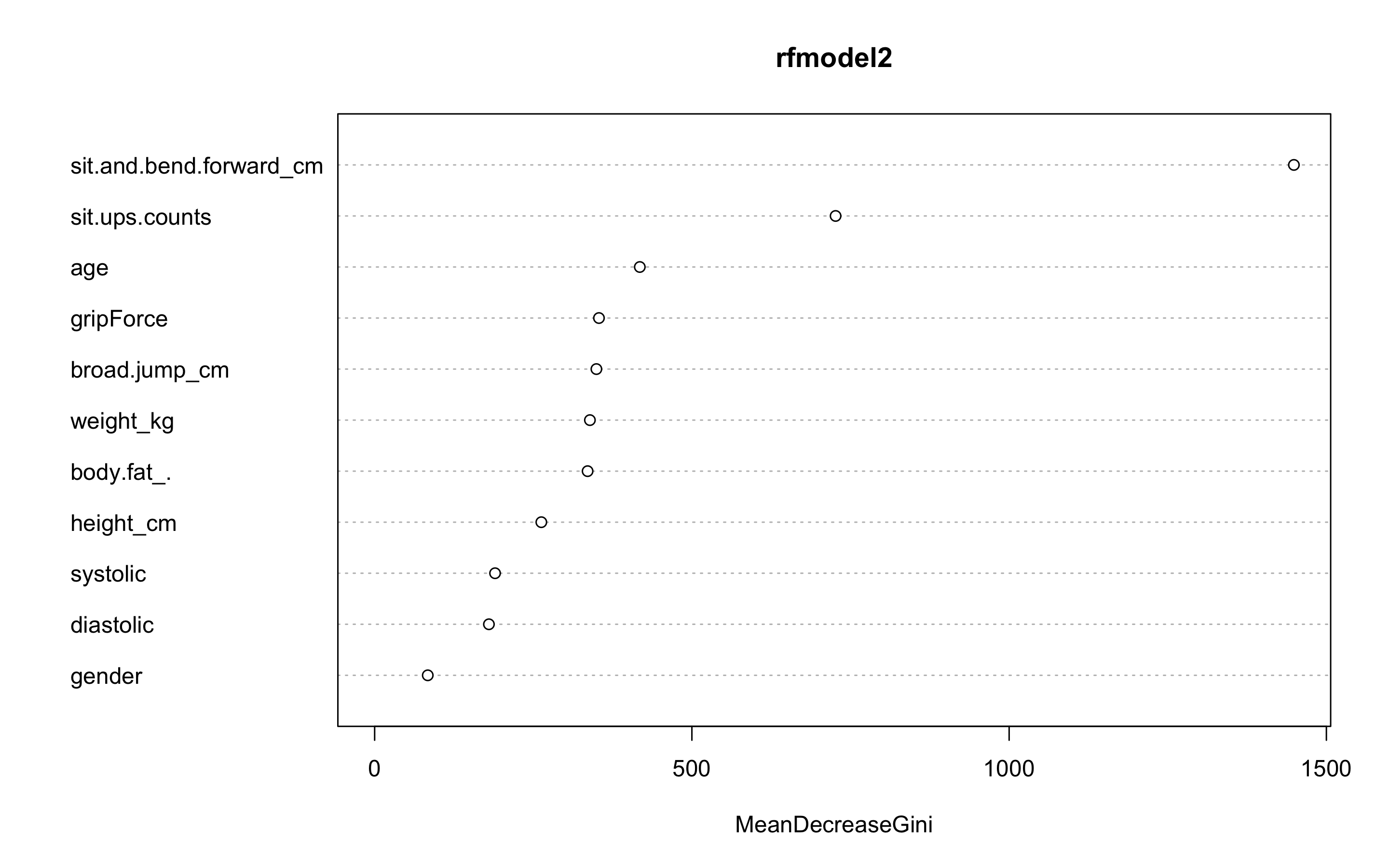
sit.and.bend.forward_cm변수와 sit.ups.counts 변수가 가장 중요한 변수인 것을 볼 수 있다.
익스트림 그레디언트 부스트
- 다음으로 익스트림 그레디언트 부스트 모델을 만들어 보자.
- scaled_train_dummy데이터와 scaled_test_dummy데이터를 사용하자.
- 부스트 기법을 사용하기 위해서는 여러 인자값들을 세부 조정해야 한다.
- 그리드를 만들어 보자.
- 각 인자값들은 다음과 같다.
| 인자 | Description |
|---|---|
| nrounds | 최대 반복 횟수(최종 모형에서의 트리 수) |
| colsample_bytree | 트리를 생성할 때 표본 추출할 피처 수(비율로 표시됨), 기본값은 1 |
| min_child_weight | 부스트되는 트리에서 최소 가중값, 기본값은 1 |
| eta | 학습 속도, 해법에 관한 각 트리의 기여도를 의미, 기본값은 0.3 |
| gamma | 트리에서 다른 leaf 분할을 하기 위해 필요한 최소 손실 감소 |
| subsample | 데이터 관찰값의 비율, 기본값은 1 |
| max_depth | 개별 트리의 최대 깊이 |
> grid <- expand.grid(nrounds = c(350, 550),
+                     colsample_bytree = 1,
+                     min_child_weight = 1,
+                     eta = c(0.01, 0.1, 0.3),
+                     gamma = c(0.5, 0.25),
+                     subsample = 0.5,
+                     max_depth = c(2, 3, 4)
+ )- trainControl인자를 조정한다. 여기서는 5-fold 교차검증을 사용할 것이다.
> cntrl <- trainControl(method = 'cv',
+                       number = 5,
+                       verboseIter = TRUE,
+                       returnData = FALSE,
+ returnResamp = 'final')- train()을 사용해 train데이터를 학습시킨다.
> train.xgb <- train(x = scaled_train_dummy[, 1:12],
                     y = scaled_train_dummy[, 13],
                     trControl = cntrl,
                     tuneGrid = grid,
                     method = 'xgbTree')
Fold1: eta=0.01, max_depth=2, gamma=0.25, colsample_bytree=1, min_child_weight=1, subsample=0.5, nrounds=550
[19:57:05] WARNING: amalgamation/../src/c_api/c_api.cc:718: `ntree_limit` is deprecated, use `iteration_range` instead.
.
.
.
- Fold5: eta=0.30, max_depth=4, gamma=0.50, colsample_bytree=1, min_child_weight=1, subsample=0.5, nrounds=550
Aggregating results
Selecting tuning parameters
Fitting nrounds = 350, max_depth = 3, eta = 0.1, gamma = 0.25, colsample_bytree = 1, min_child_weight = 1, subsample = 0.5 on full training set
상당히 긴 출력이 나오기 때문에 중간의 출력은 생략했다.
최적 인자들의 조합으로 nrounds = 350, max_depth = 3, eta = 0.1, gamma = 0.25, colsample_bytree = 1, min_child_weight = 1, subsample = 0.5이 선택되었다.
- xgb.train()에서 사용할 인자 목록을 생성하고, 데이터 프레임을 입력피처의 행렬과 숫자 레이블의 목록으로 변환한다. 그런 다음, 피처와 식별값을 xgb.DMatrix에서 사용할 입력값으로 변환한다.
> param <- list(objective = 'binary:logistic',
+               booster = 'gbtree',
+               eval_metric = 'error',
+               eta = 0.1,
+               max_depth = 3,
+               subsample = 0.5,
+               colsample_bytree = 1,
+               gamma = 0.25)
> x <- as.matrix(scaled_train_dummy[, 1:12])
> y <- ifelse(scaled_train_dummy$class == 'Good', 1, 0)
> train.mat <- xgb.DMatrix(data = x, label = y)- 이제 모형을 만들어 보자.
> set.seed(321)
> xgb.fit <- xgb.train(params = param, data = train.mat, nrounds = 350)- test데이터에 관한 결과를 보기 전에 변수 중요도를 그려 검토해보자.
- 항목은 gain, cover, frequency 이렇게 세가지를 검사할 수 있다. gain은 피처가 트리에 미치는 정확도의 향상 정도를 나타내는 값, cover는 이 피처와 연관된 전체 관찰값의 상대 수치, frequency는 모든 트리에 관해 피처가 나타난 횟수를 백분율로 나타낸 값이다.
> impMatrix <- xgb.importance(feature_names = dimnames(x)[[2]], model = xgb.fit)
> impMatrix
                    Feature       Gain      Cover  Frequency
 1: sit.and.bend.forward_cm 0.37183214 0.16417734 0.14507103
 2:          sit.ups.counts 0.18329102 0.16162442 0.13387861
 3:                     age 0.10086544 0.12283634 0.12397762
 4:               gripForce 0.07884639 0.10694276 0.11321567
 5:               weight_kg 0.07303583 0.09829464 0.09857942
 6:              body.fat_. 0.04424628 0.08274724 0.08351270
 7:           broad.jump_cm 0.04345929 0.07631799 0.08092983
 8:                gender.F 0.03445674 0.03675565 0.02884201
 9:               height_cm 0.03177574 0.05728559 0.07920792
10:                systolic 0.01999980 0.05470798 0.05811451
11:               diastolic 0.01819134 0.03831006 0.05467068
> xgb.plot.importance(impMatrix, main = 'Gain by Feature')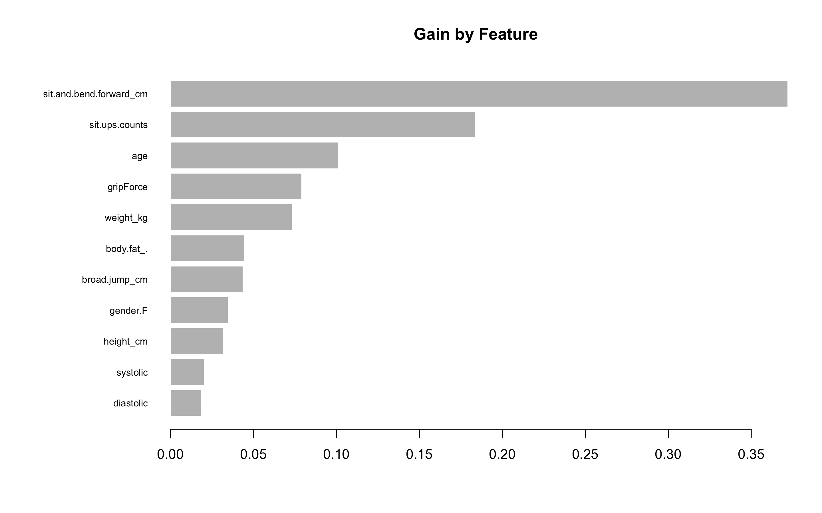
위에서 랜덤포레스트에서 봤던 변수 중요도와 마찬가지로 sit.and.bend.forward_cm변수와 sit.ups.counts 변수, age변수가 차례대로 가장 중요한 변수인 것을 볼 수 있다.
- 다음으로 테스트 세트에 관한 수행 결과를 보자.
> library(InformationValue)
> pred <- predict(xgb.fit, x)
> optimalCutoff(y, pred)
[1] 0.5472727
> testMat <- as.matrix(scaled_test_dummy[, 1:12])
> xgb.test <- predict(xgb.fit, testMat)
> y.test <- ifelse(scaled_test_dummy$class == 'Good', 1, 0)
> confusionMatrix(y.test, xgb.test, threshold = 0.5472)
     0    1
0 1704  226
1  305 1782
> 1 - misClassError(y.test, xgb.test, threshold = 0.5472)
[1] 0.8678
약 86.78%의 정확도를 보였다.
- ROC커브를 그려보자.
> plotROC(y.test, xgb.test)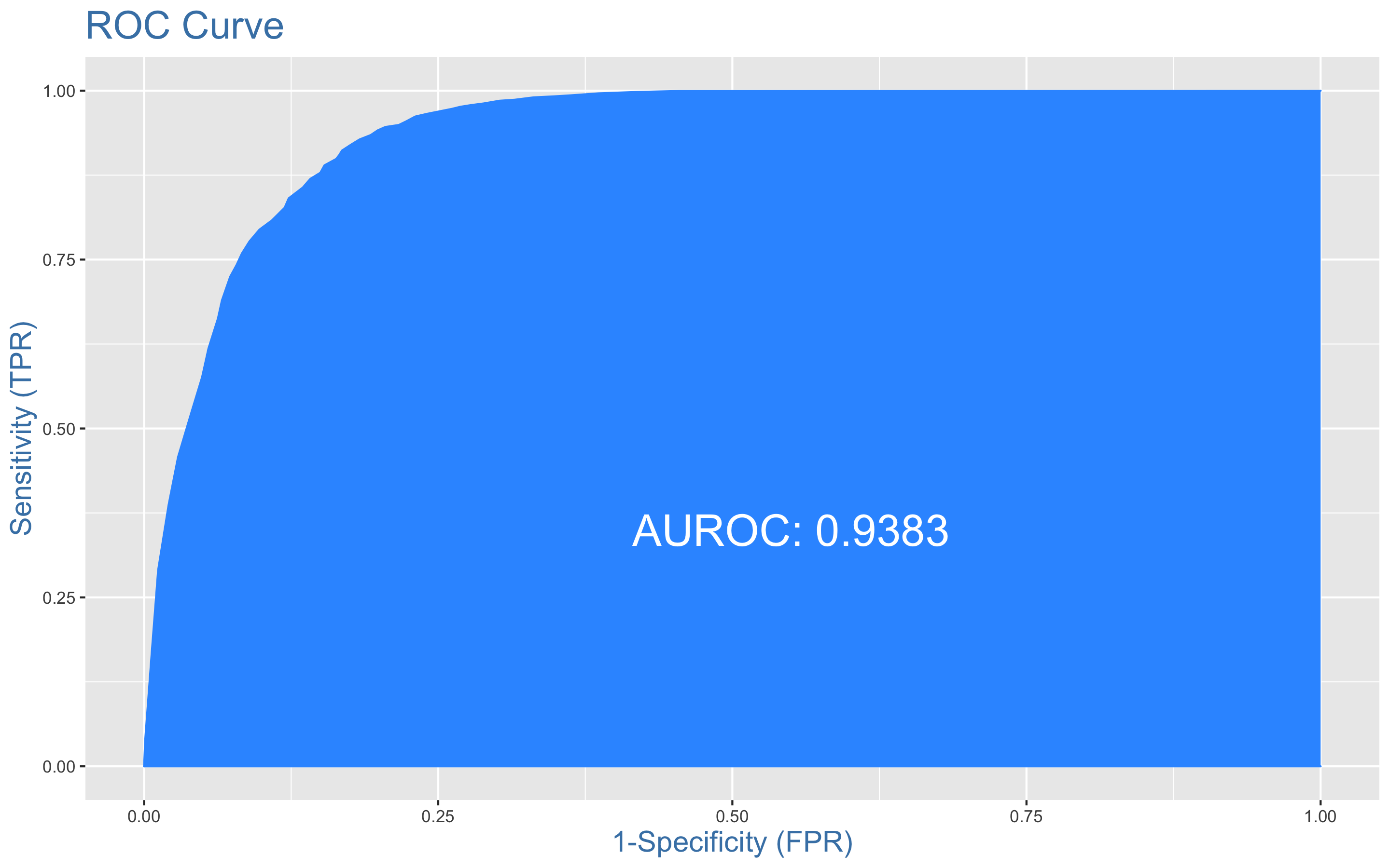
AUC는 0.938이다.
아직까지는 랜덤포레스트를 사용한 모델이 정확도 87.13%로 가장 높은 정확도를 보였다.
앙상블 분석
- 앙상블 분석을 해보자.
- 데이터는 scaled_train_dummy와 scaled_test_dummy를 사용하자.
> library(caret)
> library(MASS)
> library(caretEnsemble)
> library(caTools)
> library(mlr)
> library(ggplot2)
> library(HDclassif)
> library(reshape2)
> library(corrplot)
> library(gbm)
> library(mboost)
> control <- trainControl(method = 'cv', number = 5,
+                         savePredictions = 'final',
+                         classProbs = TRUE,
+ summaryFunction = twoClassSummary)- caretList()함수를 이용해 모형을 학습시킨다. 분류트리, 다변량 회귀 스플라인(earth), KNN을 사용해보자.
> set.seed(1234)
> models <- caretList(class ~., data = scaled_train_dummy,
+                     trControl = control,
+                     metric = 'ROC',
+                     methodList = c('rpart', 'earth', 'knn'))
> models
$rpart
CART

9376 samples
  12 predictor
   2 classes: 'Bad', 'Good'

No pre-processing
Resampling: Cross-Validated (5 fold)
Summary of sample sizes: 7502, 7501, 7500, 7500, 7501
Resampling results across tuning parameters:

  cp          ROC        Sens       Spec
  0.01258801  0.8110845  0.7208361  0.8340093
  0.10987839  0.7432973  0.5585200  0.9108469
  0.43204608  0.6281850  0.6834667  0.5729034

ROC was used to select the optimal model using the largest value.
The final value used for the model was cp = 0.01258801.

$earth
Multivariate Adaptive Regression Spline

9376 samples
  12 predictor
   2 classes: 'Bad', 'Good'

No pre-processing
Resampling: Cross-Validated (5 fold)
Summary of sample sizes: 7502, 7501, 7500, 7500, 7501
Resampling results across tuning parameters:

  nprune  ROC        Sens       Spec
   2      0.8025890  0.7099610  0.7510171
   9      0.8999423  0.7920658  0.8491607
  17      0.9101123  0.8014507  0.8549180

Tuning parameter 'degree' was held constant at a value of 1
ROC was used to select the optimal model using the largest value.
The final values used for the model were nprune = 17 and degree = 1.

$knn
k-Nearest Neighbors

9376 samples
  12 predictor
   2 classes: 'Bad', 'Good'

No pre-processing
Resampling: Cross-Validated (5 fold)
Summary of sample sizes: 7502, 7501, 7500, 7500, 7501
Resampling results across tuning parameters:

  k  ROC        Sens       Spec
  5  0.8827860  0.7381112  0.8869249
  7  0.8935599  0.7351262  0.8988700
  9  0.8990740  0.7374700  0.9056984

ROC was used to select the optimal model using the largest value.
The final value used for the model was k = 9.

attr(,"class")
[1] "caretList"- 모형끼리 상호연관성이 어떤지 살펴보자.
> modelCor(resamples(models))
          rpart     earth       knn
rpart 1.0000000 0.7959453 0.5528002
earth 0.7959453 1.0000000 0.9425428
knn   0.5528002 0.9425428 1.0000000
rpart와 earth, earth와 knn의 상호연관성이 상당히 높아보인다.
효과적인 앙상블을 위해서는 상호연관성이 높지 않은 것이 좋다.
- 다른 모델 조합으로 앙상블을 다시 시도해보자.
> set.seed(1234)
> models_2 <- caretList(class ~., data = scaled_train_dummy,
                      trControl = control,
                      metric = 'ROC',
                      methodList = c('rpart', 'knn', 'nnet'))
> modelCor(resamples(models_2))
          rpart       knn      nnet
rpart 1.0000000 0.3002102 0.4326137
knn   0.3002102 1.0000000 0.6547422
nnet  0.4326137 0.6547422 1.0000000
이 정도면 괜찮은 것으로 보인다.
- stack으로 로지스틱 회귀 모형을 쌓아보자.
- 이를 위해 데이터 프레임 안의 테스트 세트에서 'Good'값에 관한 예측값을 얻어오자.
> model_preds <- lapply(models_2, predict, newdata = scaled_test_dummy, type = 'prob')
> model_preds <- lapply(model_preds, function(x) x[, 'Good'])
> model_preds <- data.frame(model_preds)- caretStack()함수를 이용해 모형을 쌓는다.
> stack <- caretStack(models_2, mothod = 'glm', metric = 'ROC',
                    trControl = trainControl(
                      method = 'boot', number = 5,
                      savePredictions = 'final',
                      classProbs = TRUE,
                      summaryFunction = twoClassSummary
                    ))
> prob <- 1 - predict(stack, newdata = scaled_test_dummy, type = 'prob')
> model_preds$ensemble <- prob
> colAUC(model_preds, scaled_test_dummy$class)
                 rpart       knn      nnet  ensemble
Bad vs. Good 0.7942167 0.8971699 0.9343864 0.9144205
앙상블한 모형보다 nnet을 단독 사용한 모형의 AUC가 더 높게 나왔다.
Conclusion
KNN, SVM, 랜덤포레스트, 익스트림 그레디언트 부스트, 앙상블 분석까지 총 5개 유형의 모형을 만들었다.
그렇다면 위 5개의 모형 중 어떤 모형을 선택해야 하는가?
우선 앙상블 분석을 먼저 제외하겠다. 앙상블한 모형이 단독 모형보다 AUC가 낮게 나왔을 뿐더러 앙상블 모델을 만드는 데 많은 시간이 소요되고, 또한 모델간의 상관관계가 높다면 앙상블에 사용된 모델을 바꿔줘야 한다. 상관관계가 높지 않은 모델끼리 stack한다 해도 모델이 유의하지 않다면 처음으로 돌아가 모델 조합을 바꿔줘야 한다.
다음으로 KNN모형을 제외하겠다. 다양한 하이퍼 파라미터 조합으로 모형을 만들었음에도 불구하고 가장 낮은 정확도와 카파통계량을 보였기 때문이다.
또한 SVM모델도 제외하겠다. 다양한 커널함수와 하이퍼파라미터를 조합했지만 랜덤포레스트보다 낮은 성능을 보였고, 소요 시간 또한 상당히 오래걸렸기 때문이다.
나는 최종 모형으로 익스트림 그레디언트 부스트 모형을 선택하겠다. 랜덤포레스트와 거의 유사한 성능을 보였으며, 다양한 하이퍼파라미터 조합과 5-fold 교차검증을 사용해 과적합을 방지할 수 있기 때문이다.
또한 변수 중요도 plot과 매트릭스를 볼 수 있어서 어떤 예측변수가 결과변수에 더 큰 영향을 주는지 눈으로 확인할 수 있어 이해관계자들에게 설명해주거나 설득을 해야 할때 다른 모델들보다 더 용이한 모델이라고 생각한다.
사용한 패키지
pastecs, psych, GGally, reshape2, caret, ggplot2, gridExtra, gapminder, dplyr, Boruta, class, kknn, e1071, MASS, kernlab, corrplot, rpart, partykit, genridge, randomForest, xgboost, caretEnsemble, caTools, mlr, HDclassif, gbm, mboost