Bank Marketing Data Set
데이터 출처
The data is related with direct marketing campaigns of a Portuguese banking institution. The marketing campaigns were based on phone calls. Often, more than one contact to the same client was required, in order to access if the product (bank term deposit) would be ('yes') or not ('no') subscribed
데이터는 총 21개의 칼럼과 41188개의 rows로 구성
| Header | Description |
|---|---|
| age | numeric |
| job | type of job (categorical: 'admin.','blue-collar','entrepreneur','housemaid','management','retired','self-employed','services','student','technician','unemployed','unknown') |
| marital | marital status (categorical: 'divorced','married','single','unknown'; note: 'divorced' means divorced or widowed) |
| education | (categorical: 'basic.4y','basic.6y','basic.9y','high.school','illiterate','professional.course','university.degree','unknown') |
| default | has credit in default? (categorical: 'no','yes','unknown') |
| housing | has housing loan? (categorical: 'no','yes','unknown') |
| loan | has personal loan? (categorical: 'no','yes','unknown') |
| contact | contact communication type (categorical: 'cellular','telephone') |
| month | last contact month of year (categorical: 'jan', 'feb', 'mar', ..., 'nov', 'dec') |
| day_of_week | last contact day of the week (categorical: 'mon','tue','wed','thu','fri') |
| duration | last contact duration, in seconds (numeric). Important note: this attribute highly affects the output target (e.g., if duration=0 then y='no'). Yet, the duration is not known before a call is performed. Also, after the end of the call y is obviously known. Thus, this input should only be included for benchmark purposes and should be discarded if the intention is to have a realistic predictive model. |
| campaign | number of contacts performed during this campaign and for this client (numeric, includes last contact) |
| pdays | number of days that passed by after the client was last contacted from a previous campaign (numeric; 999 means client was not previously contacted) |
| previous | number of contacts performed before this campaign and for this client (numeric) |
| poutcome | outcome of the previous marketing campaign (categorical: 'failure','nonexistent','success') |
| emp.var.rate | employment variation rate - quarterly indicator (numeric) |
| cons.price.idx | consumer price index - monthly indicator (numeric) |
| cons.conf.idx | consumer confidence index - monthly indicator (numeric) |
| euribor3m | euribor 3 month rate - daily indicator (numeric) |
| nr.employed | number of employees - quarterly indicator (numeric) |
| y | has the client subscribed a term deposit? (binary: 'yes','no') |
EDA
- 데이터 구조 파악
> df <- read.csv('bank-additional-full.csv', sep = ';', stringsAsFactors = TRUE)
> dim(df)
[1] 41188    21
> head(df)
  age       job marital   education default housing loan   contact month
1  56 housemaid married    basic.4y      no      no   no telephone   may
2  57  services married high.school unknown      no   no telephone   may
3  37  services married high.school      no     yes   no telephone   may
4  40    admin. married    basic.6y      no      no   no telephone   may
5  56  services married high.school      no      no  yes telephone   may
6  45  services married    basic.9y unknown      no   no telephone   may
  day_of_week duration campaign pdays previous    poutcome emp.var.rate
1         mon      261        1   999        0 nonexistent          1.1
2         mon      149        1   999        0 nonexistent          1.1
3         mon      226        1   999        0 nonexistent          1.1
4         mon      151        1   999        0 nonexistent          1.1
5         mon      307        1   999        0 nonexistent          1.1
6         mon      198        1   999        0 nonexistent          1.1
  cons.price.idx cons.conf.idx euribor3m nr.employed  y
1         93.994         -36.4     4.857        5191 no
2         93.994         -36.4     4.857        5191 no
3         93.994         -36.4     4.857        5191 no
4         93.994         -36.4     4.857        5191 no
5         93.994         -36.4     4.857        5191 no
6         93.994         -36.4     4.857        5191 no
> str(df)
'data.frame':	41188 obs. of  21 variables:
 $ age           : int  56 57 37 40 56 45 59 41 24 25 ...
 $ job           : Factor w/ 12 levels "admin.","blue-collar",..: 4 8 8 1 8 8 1 2 10 8 ...
 $ marital       : Factor w/ 4 levels "divorced","married",..: 2 2 2 2 2 2 2 2 3 3 ...
 $ education     : Factor w/ 8 levels "basic.4y","basic.6y",..: 1 4 4 2 4 3 6 8 6 4 ...
 $ default       : Factor w/ 3 levels "no","unknown",..: 1 2 1 1 1 2 1 2 1 1 ...
 $ housing       : Factor w/ 3 levels "no","unknown",..: 1 1 3 1 1 1 1 1 3 3 ...
 $ loan          : Factor w/ 3 levels "no","unknown",..: 1 1 1 1 3 1 1 1 1 1 ...
 $ contact       : Factor w/ 2 levels "cellular","telephone": 2 2 2 2 2 2 2 2 2 2 ...
 $ month         : Factor w/ 10 levels "apr","aug","dec",..: 7 7 7 7 7 7 7 7 7 7 ...
 $ day_of_week   : Factor w/ 5 levels "fri","mon","thu",..: 2 2 2 2 2 2 2 2 2 2 ...
 $ duration      : int  261 149 226 151 307 198 139 217 380 50 ...
 $ campaign      : int  1 1 1 1 1 1 1 1 1 1 ...
 $ pdays         : int  999 999 999 999 999 999 999 999 999 999 ...
 $ previous      : int  0 0 0 0 0 0 0 0 0 0 ...
 $ poutcome      : Factor w/ 3 levels "failure","nonexistent",..: 2 2 2 2 2 2 2 2 2 2 ...
 $ emp.var.rate  : num  1.1 1.1 1.1 1.1 1.1 1.1 1.1 1.1 1.1 1.1 ...
 $ cons.price.idx: num  94 94 94 94 94 ...
 $ cons.conf.idx : num  -36.4 -36.4 -36.4 -36.4 -36.4 -36.4 -36.4 -36.4 -36.4 -36.4 ...
 $ euribor3m     : num  4.86 4.86 4.86 4.86 4.86 ...
 $ nr.employed   : num  5191 5191 5191 5191 5191 ...
 $ y             : Factor w/ 2 levels "no","yes": 1 1 1 1 1 1 1 1 1 1 ...
> summary(df)
      age                 job            marital
 Min.   :17.00   admin.     :10422   divorced: 4612
 1st Qu.:32.00   blue-collar: 9254   married :24928
 Median :38.00   technician : 6743   single  :11568
 Mean   :40.02   services   : 3969   unknown :   80
 3rd Qu.:47.00   management : 2924
 Max.   :98.00   retired    : 1720
                 (Other)    : 6156
               education        default         housing           loan
 university.degree  :12168   no     :32588   no     :18622   no     :33950
 high.school        : 9515   unknown: 8597   unknown:  990   unknown:  990
 basic.9y           : 6045   yes    :    3   yes    :21576   yes    : 6248
 professional.course: 5243
 basic.4y           : 4176
 basic.6y           : 2292
 (Other)            : 1749
      contact          month       day_of_week    duration
 cellular :26144   may    :13769   fri:7827    Min.   :   0.0
 telephone:15044   jul    : 7174   mon:8514    1st Qu.: 102.0
                   aug    : 6178   thu:8623    Median : 180.0
                   jun    : 5318   tue:8090    Mean   : 258.3
                   nov    : 4101   wed:8134    3rd Qu.: 319.0
                   apr    : 2632               Max.   :4918.0
                   (Other): 2016
    campaign          pdays          previous            poutcome
 Min.   : 1.000   Min.   :  0.0   Min.   :0.000   failure    : 4252
 1st Qu.: 1.000   1st Qu.:999.0   1st Qu.:0.000   nonexistent:35563
 Median : 2.000   Median :999.0   Median :0.000   success    : 1373
 Mean   : 2.568   Mean   :962.5   Mean   :0.173
 3rd Qu.: 3.000   3rd Qu.:999.0   3rd Qu.:0.000
 Max.   :56.000   Max.   :999.0   Max.   :7.000

  emp.var.rate      cons.price.idx  cons.conf.idx     euribor3m
 Min.   :-3.40000   Min.   :92.20   Min.   :-50.8   Min.   :0.634
 1st Qu.:-1.80000   1st Qu.:93.08   1st Qu.:-42.7   1st Qu.:1.344
 Median : 1.10000   Median :93.75   Median :-41.8   Median :4.857
 Mean   : 0.08189   Mean   :93.58   Mean   :-40.5   Mean   :3.621
 3rd Qu.: 1.40000   3rd Qu.:93.99   3rd Qu.:-36.4   3rd Qu.:4.961
 Max.   : 1.40000   Max.   :94.77   Max.   :-26.9   Max.   :5.045

  nr.employed     y
 Min.   :4964   no :36548
 1st Qu.:5099   yes: 4640
 Median :5191
 Mean   :5167
 3rd Qu.:5228
 Max.   :5228

> sum(is.na(df))
[1] 0
NA값은 없으며, 결과변수인 'y'가 no는 36548건, yes는 4640으로 불균형 데이터이다.
- 위의 변수 설명을 보면 'duration'변수는 결과변수에 너무 큰 영향을 미치는 변수로써 모델을 만들 때 삭제하라고 조언되어 있으므로 삭제한다.
> df <- df[, -11]
> str(df)
'data.frame':	41188 obs. of  20 variables:
 $ age           : int  56 57 37 40 56 45 59 41 24 25 ...
 $ job           : Factor w/ 12 levels "admin.","blue-collar",..: 4 8 8 1 8 8 1 2 10 8 ...
 $ marital       : Factor w/ 4 levels "divorced","married",..: 2 2 2 2 2 2 2 2 3 3 ...
 $ education     : Factor w/ 8 levels "basic.4y","basic.6y",..: 1 4 4 2 4 3 6 8 6 4 ...
 $ default       : Factor w/ 3 levels "no","unknown",..: 1 2 1 1 1 2 1 2 1 1 ...
 $ housing       : Factor w/ 3 levels "no","unknown",..: 1 1 3 1 1 1 1 1 3 3 ...
 $ loan          : Factor w/ 3 levels "no","unknown",..: 1 1 1 1 3 1 1 1 1 1 ...
 $ contact       : Factor w/ 2 levels "cellular","telephone": 2 2 2 2 2 2 2 2 2 2 ...
 $ month         : Factor w/ 10 levels "apr","aug","dec",..: 7 7 7 7 7 7 7 7 7 7 ...
 $ day_of_week   : Factor w/ 5 levels "fri","mon","thu",..: 2 2 2 2 2 2 2 2 2 2 ...
 $ campaign      : int  1 1 1 1 1 1 1 1 1 1 ...
 $ pdays         : int  999 999 999 999 999 999 999 999 999 999 ...
 $ previous      : int  0 0 0 0 0 0 0 0 0 0 ...
 $ poutcome      : Factor w/ 3 levels "failure","nonexistent",..: 2 2 2 2 2 2 2 2 2 2 ...
 $ emp.var.rate  : num  1.1 1.1 1.1 1.1 1.1 1.1 1.1 1.1 1.1 1.1 ...
 $ cons.price.idx: num  94 94 94 94 94 ...
 $ cons.conf.idx : num  -36.4 -36.4 -36.4 -36.4 -36.4 -36.4 -36.4 -36.4 -36.4 -36.4 ...
 $ euribor3m     : num  4.86 4.86 4.86 4.86 4.86 ...
 $ nr.employed   : num  5191 5191 5191 5191 5191 ...
$ y : Factor w/ 2 levels "no","yes": 1 1 1 1 1 1 1 1 1 1 ...- EDA에 필요한 패키지들을 한꺼번에 불러보자
> library(DMwR2)
> library(pastecs)
> library(psych)
> library(caret)
> library(ggplot2)
> library(GGally)
> library(smotefamily)
> library(naniar)
> library(reshape2)
> library(gridExtra)
> library(gapminder)
> library(dplyr)
> library(PerformanceAnalytics)
> library(FSelector)
> library(Boruta)
> library(ROSE)- 탐색적 분석으로 첨도 및 왜도를 그려보자.
> describeBy(df[, -c(2, 3, 4, 5, 6, 7, 8, 9, 10, 14, 20)], df$y, mat = FALSE)

 Descriptive statistics by group
group: no
               vars     n    mean     sd  median trimmed   mad     min     max  range  skew kurtosis   se
age               1 36548   39.91   9.90   38.00   39.31 10.38   17.00   95.00  78.00  0.65     0.36 0.05
campaign          2 36548    2.63   2.87    2.00    2.03  1.48    1.00   56.00  55.00  4.68    35.21 0.02
pdays             3 36548  984.11 120.66  999.00  999.00  0.00    0.00  999.00 999.00 -7.98    61.71 0.63
previous          4 36548    0.13   0.41    0.00    0.02  0.00    0.00    7.00   7.00  4.05    23.81 0.00
emp.var.rate      5 36548    0.25   1.48    1.10    0.44  0.44   -3.40    1.40   4.80 -0.91    -0.75 0.01
cons.price.idx    6 36548   93.60   0.56   93.92   93.61  0.70   92.20   94.77   2.57 -0.24    -0.82 0.00
cons.conf.idx     7 36548  -40.59   4.39  -41.80  -40.61  6.52  -50.80  -26.90  23.90  0.25    -0.48 0.02
euribor3m         8 36548    3.81   1.64    4.86    4.02  0.16    0.63    5.04   4.41 -0.94    -1.01 0.01
nr.employed       9 36548 5176.17  64.57 5195.80 5185.86 47.89 4963.60 5228.10 264.50 -1.21     0.54 0.34
---------------------------------------------------------------------------------------
group: yes
               vars    n    mean     sd  median trimmed    mad     min     max  range  skew kurtosis   se
age               1 4640   40.91  13.84   37.00   39.42  11.86   17.00   98.00  81.00  1.00     0.67 0.20
campaign          2 4640    2.05   1.67    2.00    1.71   1.48    1.00   23.00  22.00  3.38    19.32 0.02
pdays             3 4640  792.04 403.41  999.00  864.77   0.00    0.00  999.00 999.00 -1.44     0.06 5.92
previous          4 4640    0.49   0.86    0.00    0.30   0.00    0.00    6.00   6.00  2.13     5.26 0.01
emp.var.rate      5 4640   -1.23   1.62   -1.80   -1.29   1.63   -3.40    1.40   4.80  0.56    -0.99 0.02
cons.price.idx    6 4640   93.35   0.68   93.20   93.35   0.82   92.20   94.77   2.57  0.12    -1.06 0.01
cons.conf.idx     7 4640  -39.79   6.14  -40.40  -40.03   8.30  -50.80  -26.90  23.90  0.26    -0.79 0.09
euribor3m         8 4640    2.12   1.74    1.27    1.95   0.73    0.63    5.04   4.41  0.89    -1.09 0.03
nr.employed       9 4640 5095.12  87.57 5099.10 5093.70 134.03 4963.60 5228.10 264.50  0.28    -1.20 1.29
'campaign', 'pdays', 'previous'변수는 첨도(kurtosis)와 왜도(skewness)가 0에서 멀어 정규분포에서 크게 벗어난 것으로 보인다.
- 그래프로 변수별 분포를 확인해보자.
- 예측변수가 19개나 되므로 수치형 변수와 팩터형 변수를 따로 보자.
- 우선 수치형 변수부터 보자
ggpairs(df, columns = c(1, 11, 12, 13, 15, 16, 17, 18, 19), aes(colour = y, alpha = 0.4))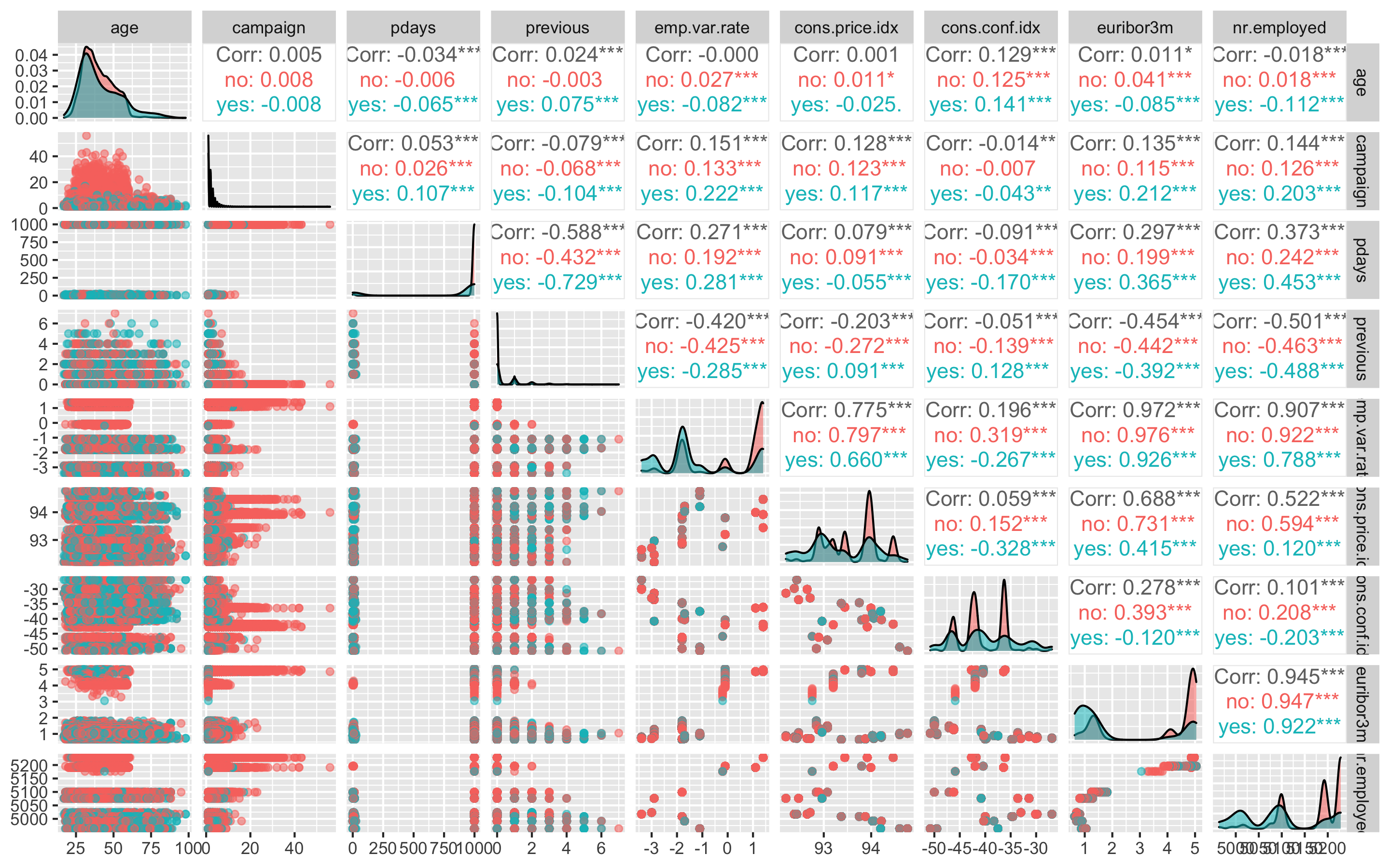
결과변수 'y'의 no가 분홍색이고, yes가 하늘색이다.
'age', 'campaign'변수는 는 yes나 no나 비슷한 분포를 보이지만 나머지 변수들에서는 yes와 no가 차이나는 분포를 보이고 있다.
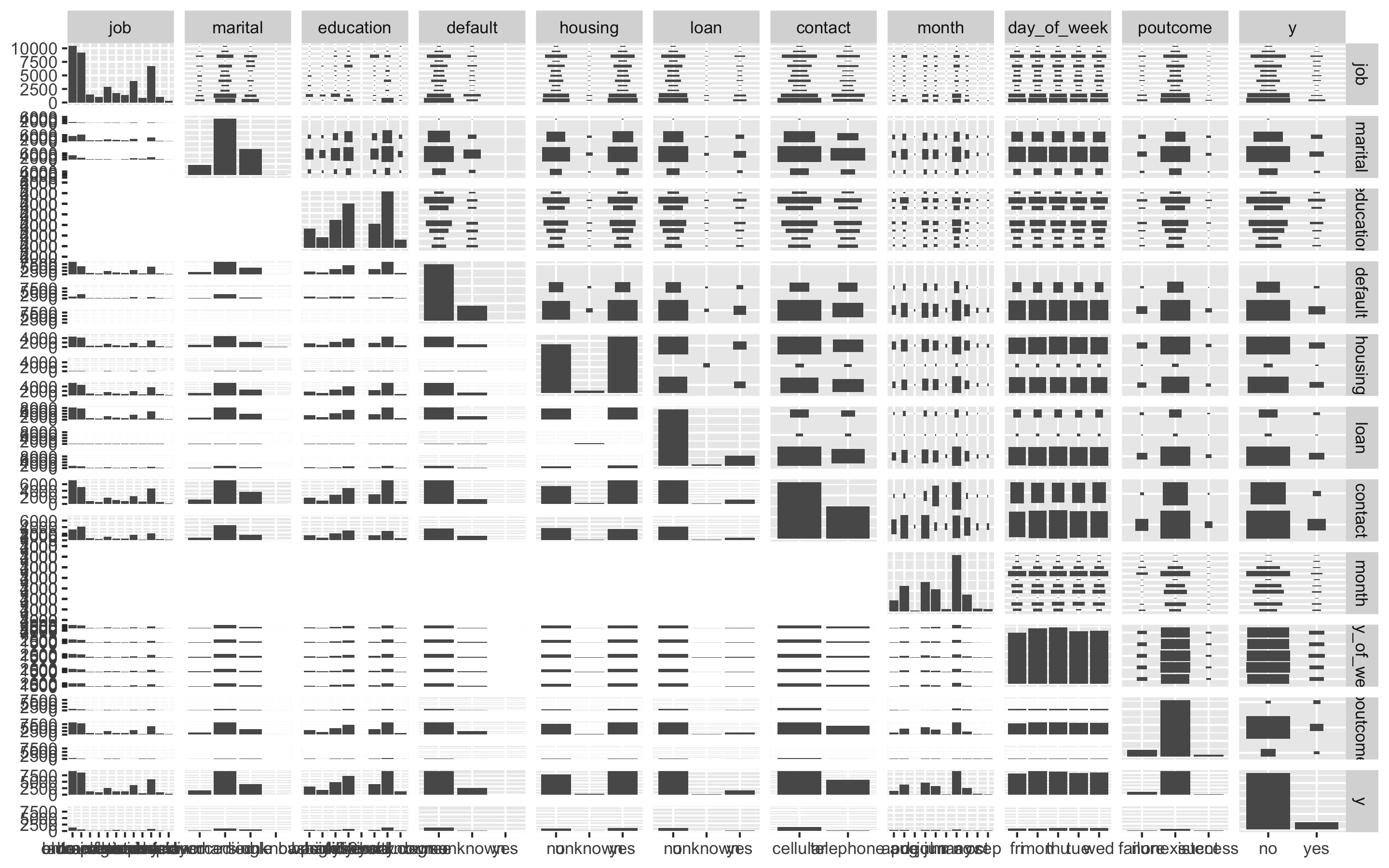
- 팩터형 변수들을 보자
ggpairs(df, columns = c(2, 3, 4, 5, 6, 7, 8, 9, 10, 14), aes(colour = y, alpha = 0.4))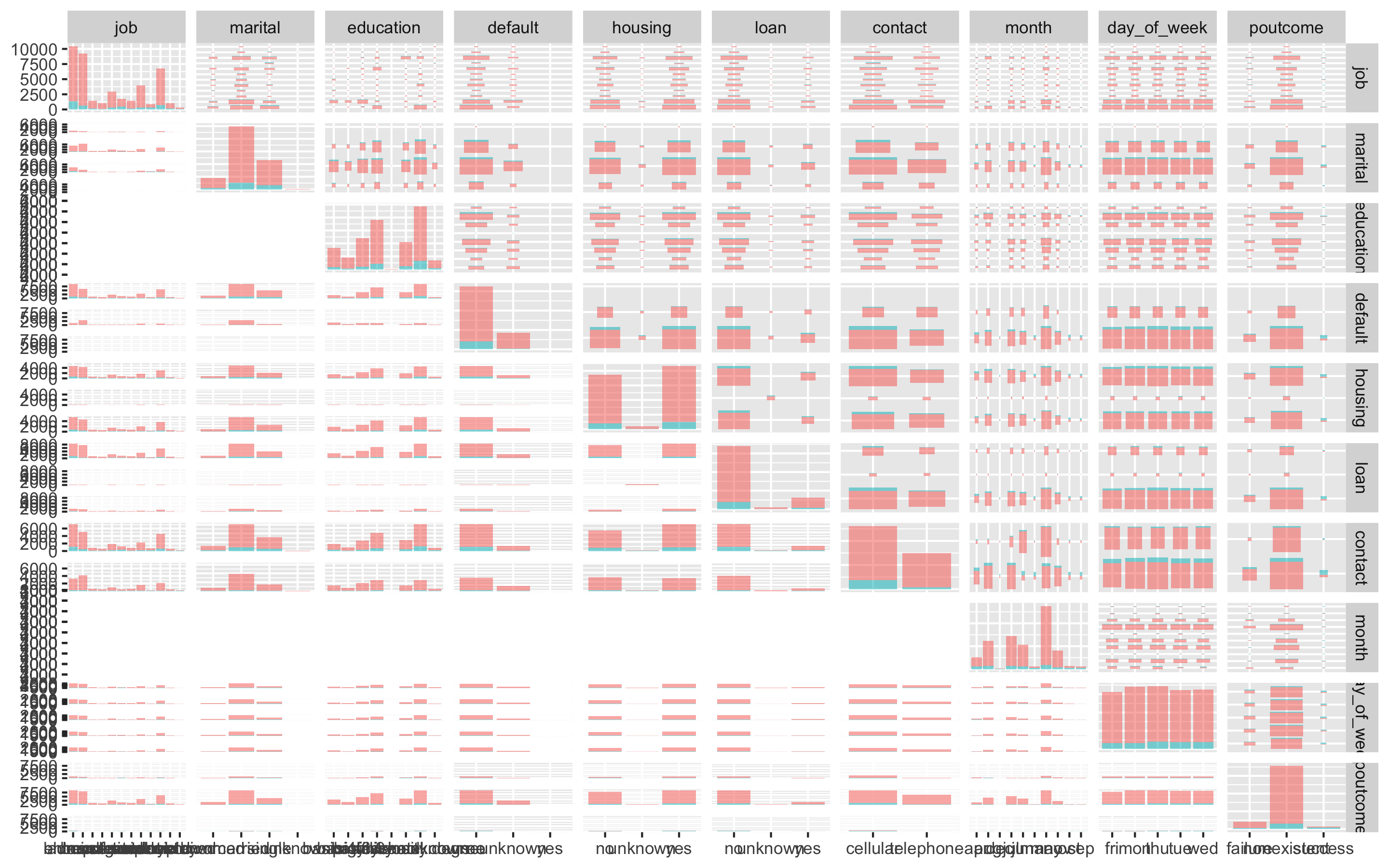
결과변수 'y'의 no가 분홍색이고, yes가 하늘색이다.
오른쪽 위부터 왼쪽 아래로 오는 대각선의 그래프를 보면 되는데, 'day_of_week'를 제외한 모든 변수들이 불균형한 분포를 보이고 있고, 특히 'loan'변수와 'poutcome'변수의 불균형이 심각해 보인다.
- 더 자세히 살펴보기 위해 수치형 변수들의 boxplot을 그려보자.
- 원래 데이터의 범위가 변수별로 차이나므로 평균이 0, 분산이 1이 되도록 스케일링 해주고, 데이터를 wide형식에서 long형식으로 바꿔준다.
> df_numeric <- df[, c(1, 11, 12, 13, 15, 16, 17, 18, 19, 20)]
> model_scale <- preProcess(df_numeric, method = c('center', 'scale'))
> scaled_df <- predict(model_scale, df_numeric)
> melt_df <- melt(scaled_df, id.vars = 'y')
> head(melt_df)
   y variable        value
1 no      age  1.533015677
2 no      age  1.628973456
3 no      age -0.290182119
4 no      age -0.002308783
5 no      age  1.533015677
6 no age 0.477480111- boxplot을 그려보자
> p1 <- ggplot(melt_df, aes(x = variable, y = value, fill = y)) + geom_boxplot()
> p1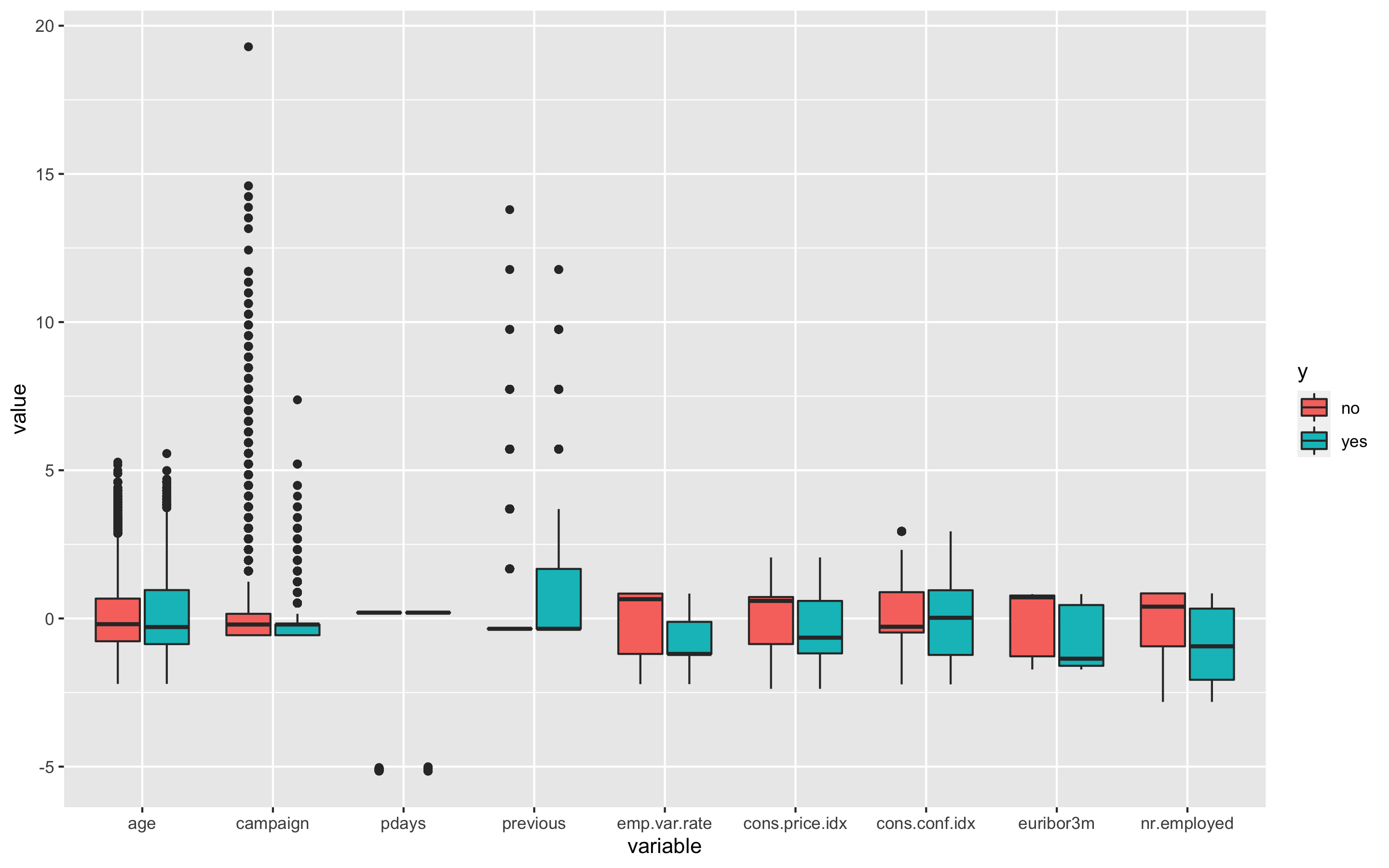
'age', 'campaign', 'pdays', 'previous', 'cons.conf.idx'변수에 boxplot상의 이상치들이 보인다.
age변수부터 보면 아까 summary(df)에서 봤듯이 최솟값이 17, 최댓값이 98이었다. 마케팅 캠페인에서 정기예금적금에 가입하는데 17살과 98살이 이상치로 보이지는 않으므로 이상치라고 볼 수 없다.
campaign변수는 이 캠페인 동안 및 이 클라이언트에 대해 수행된 컨택 수인데 최솟값이 1, 최댓값이 56이므로 이 또한 이상치로 보이지 않는다.
pdays변수는 이전 캠페인에서 클라이언트가 마지막으로 컨택된 후 경과한 일 수(숫자, 999는 클라이언트가 연결되지 않았음을 의미)를 의미하는데, 최소값이 0, 최댓값이 999로 오늘 연락을 받아서 경과일 수가 0일인 고객이 있을 수 있는 것이므로 이 또한 이상치라고 볼 수 없다.
previous변수는 이 캠페인 이전에 이 고객에 대해 수행된 컨택 수인데 최솟값이 0, 최댓값이 7이므로 역시 이상치라고 볼 수 없다.
cons.conf.idx변수는 소비자 신뢰 지수 - 월별 지표(숫자)를 나타내는데 최솟값이 -50.8, 최댓값이 -26.9로 역시 이상치로 보이지 않는다.
이처럼 boxplot상에서는 이상치로 보일지라도 자세히 뜯어보면 이상치가 아닌 경우들이 존재하므로 주의가 필요하다.
- 변수들의 상관관계를 확인하자
> str(df_numeric)
'data.frame':	41188 obs. of  10 variables:
 $ age           : int  56 57 37 40 56 45 59 41 24 25 ...
 $ campaign      : int  1 1 1 1 1 1 1 1 1 1 ...
 $ pdays         : int  999 999 999 999 999 999 999 999 999 999 ...
 $ previous      : int  0 0 0 0 0 0 0 0 0 0 ...
 $ emp.var.rate  : num  1.1 1.1 1.1 1.1 1.1 1.1 1.1 1.1 1.1 1.1 ...
 $ cons.price.idx: num  94 94 94 94 94 ...
 $ cons.conf.idx : num  -36.4 -36.4 -36.4 -36.4 -36.4 -36.4 -36.4 -36.4 -36.4 -36.4 ...
 $ euribor3m     : num  4.86 4.86 4.86 4.86 4.86 ...
 $ nr.employed   : num  5191 5191 5191 5191 5191 ...
 $ y             : Factor w/ 2 levels "no","yes": 1 1 1 1 1 1 1 1 1 1 ...
> df_numeric <- df_numeric[, -10]
> cor_df <- cor(df_numeric)
> chart.Correlation(df_numeric, histogram = TRUE, pch = 19, method = 'pearson')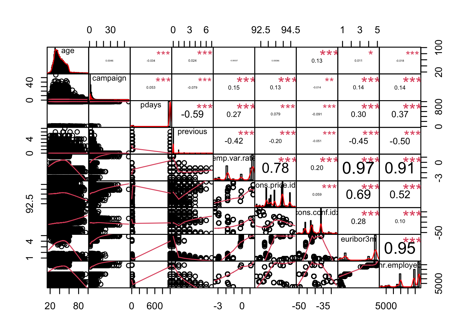
보통 상관계수의 절댓값이 0.7보다 크면 강한 상관관계가 있다고 보고, 0.3보다 크면 약한 상관관계가 있다고 본다. 상관계수가 0.3보다 작으면 일반적으로 상관관계가 없다고 해석한다. 독립변수 간에 선형 상관관계가 존재하는 경우 다중공선성이 있다고 얘기하는데, 다중공선성이 있으면 독립변수 간에 선형상관관계가 있어서 회귀계수의 분산이 커진다. 그 결과 분석 결과가 불안정하게 되어 분석의 효과성이 감소하는 문제가 발생한다.
emp.var.rate변수와 cons.price.idx변수의 상관관계가 0.78이고, emp.var.rate변수와 euribor3m변수의 상관관계가 0.97, emp.var.rate변수와 nr.employed변수의 상관관계가 0.91, euribor3m변수와 nr.employed변수의 상관관계가 0.95로 상당히 높다.
- 상관관계의 절댓값이 0.7이상이라면 제거하자
> findCorrelation(cor_df, cutoff = 0.7)
[1] 8 5- df_numeric에서 8번째 변수와 5번째 변수는 euribor3m변수와 emp.var.rate변수이므로 이 둘을 df에서 제거한다.
> df_new <- df[, -c(18, 15)]
> str(df_new)
'data.frame':	41188 obs. of  18 variables:
 $ age           : int  56 57 37 40 56 45 59 41 24 25 ...
 $ job           : Factor w/ 12 levels "admin.","blue-collar",..: 4 8 8 1 8 8 1 2 10 8 ...
 $ marital       : Factor w/ 4 levels "divorced","married",..: 2 2 2 2 2 2 2 2 3 3 ...
 $ education     : Factor w/ 8 levels "basic.4y","basic.6y",..: 1 4 4 2 4 3 6 8 6 4 ...
 $ default       : Factor w/ 3 levels "no","unknown",..: 1 2 1 1 1 2 1 2 1 1 ...
 $ housing       : Factor w/ 3 levels "no","unknown",..: 1 1 3 1 1 1 1 1 3 3 ...
 $ loan          : Factor w/ 3 levels "no","unknown",..: 1 1 1 1 3 1 1 1 1 1 ...
 $ contact       : Factor w/ 2 levels "cellular","telephone": 2 2 2 2 2 2 2 2 2 2 ...
 $ month         : Factor w/ 10 levels "apr","aug","dec",..: 7 7 7 7 7 7 7 7 7 7 ...
 $ day_of_week   : Factor w/ 5 levels "fri","mon","thu",..: 2 2 2 2 2 2 2 2 2 2 ...
 $ campaign      : int  1 1 1 1 1 1 1 1 1 1 ...
 $ pdays         : int  999 999 999 999 999 999 999 999 999 999 ...
 $ previous      : int  0 0 0 0 0 0 0 0 0 0 ...
 $ poutcome      : Factor w/ 3 levels "failure","nonexistent",..: 2 2 2 2 2 2 2 2 2 2 ...
 $ cons.price.idx: num  94 94 94 94 94 ...
 $ cons.conf.idx : num  -36.4 -36.4 -36.4 -36.4 -36.4 -36.4 -36.4 -36.4 -36.4 -36.4 ...
 $ nr.employed   : num  5191 5191 5191 5191 5191 ...
$ y : Factor w/ 2 levels "no","yes": 1 1 1 1 1 1 1 1 1 1 ...- 분산이 0에 가까운 변수도 제거한다.
변수를 선택하는 기법 중 가장 단순한 방법은 변숫값의 분산을 보는 것이다. 예를 들어, 데이터 1000개가 있는데 이 중 990개는 변수 A의 값이 0, 10개에서 변수 A의 값이 1이라고 하자. 그러면 변수 A는 서로 다른 관찰을 구별하는 데 별 소용이 없다. 따라서 데이터 모델링에서도 그리 유용하지 않다. 이런 변수는 분산이 0에 가까우므로 분석 전에 제거해준다.
> nearZeroVar(df_new, saveMetrics = TRUE)
               freqRatio percentUnique zeroVar   nzv
age             1.054713   0.189375546   FALSE FALSE
job             1.126216   0.029134699   FALSE FALSE
marital         2.154910   0.009711566   FALSE FALSE
education       1.278823   0.019423133   FALSE FALSE
default         3.790625   0.007283675   FALSE FALSE
housing         1.158630   0.007283675   FALSE FALSE
loan            5.433739   0.007283675   FALSE FALSE
contact         1.737836   0.004855783   FALSE FALSE
month           1.919292   0.024278916   FALSE FALSE
day_of_week     1.012802   0.012139458   FALSE FALSE
campaign        1.669063   0.101971448   FALSE FALSE
pdays          90.371298   0.065553074   FALSE  TRUE
previous        7.797194   0.019423133   FALSE FALSE
poutcome        8.363829   0.007283675   FALSE FALSE
cons.price.idx  1.161257   0.063125182   FALSE FALSE
cons.conf.idx   1.161257   0.063125182   FALSE FALSE
nr.employed     1.902273   0.026706808   FALSE FALSE
y               7.876724   0.004855783   FALSE FALSE
> df_new2 <- df_new[, -nearZeroVar(df_new)]
> str(df_new2)
'data.frame':	41188 obs. of  17 variables:
 $ age           : int  56 57 37 40 56 45 59 41 24 25 ...
 $ job           : Factor w/ 12 levels "admin.","blue-collar",..: 4 8 8 1 8 8 1 2 10 8 ...
 $ marital       : Factor w/ 4 levels "divorced","married",..: 2 2 2 2 2 2 2 2 3 3 ...
 $ education     : Factor w/ 8 levels "basic.4y","basic.6y",..: 1 4 4 2 4 3 6 8 6 4 ...
 $ default       : Factor w/ 3 levels "no","unknown",..: 1 2 1 1 1 2 1 2 1 1 ...
 $ housing       : Factor w/ 3 levels "no","unknown",..: 1 1 3 1 1 1 1 1 3 3 ...
 $ loan          : Factor w/ 3 levels "no","unknown",..: 1 1 1 1 3 1 1 1 1 1 ...
 $ contact       : Factor w/ 2 levels "cellular","telephone": 2 2 2 2 2 2 2 2 2 2 ...
 $ month         : Factor w/ 10 levels "apr","aug","dec",..: 7 7 7 7 7 7 7 7 7 7 ...
 $ day_of_week   : Factor w/ 5 levels "fri","mon","thu",..: 2 2 2 2 2 2 2 2 2 2 ...
 $ campaign      : int  1 1 1 1 1 1 1 1 1 1 ...
 $ previous      : int  0 0 0 0 0 0 0 0 0 0 ...
 $ poutcome      : Factor w/ 3 levels "failure","nonexistent",..: 2 2 2 2 2 2 2 2 2 2 ...
 $ cons.price.idx: num  94 94 94 94 94 ...
 $ cons.conf.idx : num  -36.4 -36.4 -36.4 -36.4 -36.4 -36.4 -36.4 -36.4 -36.4 -36.4 ...
 $ nr.employed   : num  5191 5191 5191 5191 5191 ...
$ y : Factor w/ 2 levels "no","yes": 1 1 1 1 1 1 1 1 1 1 ...- 예측변수가 16개로 아직 다소 많아 보인다.
- 랜덤포레스트를 사용해 피처를 선택해보자.
> set.seed(123)
> feature.selection <- Boruta(y ~., data = df_new2, doTrace = TRUE)
After 11 iterations, +2.6 mins:
 confirmed 14 attributes: age, campaign, cons.conf.idx, cons.price.idx, contact and 9 more;
 still have 2 attributes left.

After 15 iterations, +3.6 mins:
 rejected 2 attributes: housing, loan;
 no more attributes left.

> table(feature.selection$finalDecision)

Tentative Confirmed  Rejected
0 14 2 - 탈락(Rejected)된 변수를 제거하자.
> fNames <- getSelectedAttributes(feature.selection, withTentative = TRUE)
> fNames
 [1] "age"            "job"            "marital"        "education"
 [5] "default"        "contact"        "month"          "day_of_week"
 [9] "campaign"       "previous"       "poutcome"       "cons.price.idx"
[13] "cons.conf.idx"  "nr.employed"
> df <- df_new2[, fNames]
> dim(df)
[1] 41188    14
> df$y <- df_new2$y
예측변수가 16개에서 14개로 줄어들었다.
- 변수를 더 줄이고 싶다면 카이제곱 검정을 사용한 독립성 검정으로 변수의 가중치를 계산해 중요도가 낮은 변수를 탈락시킨다.
> cs <- chi.squared(y ~., data = df)
> cutoff.k(cs, 12)
 [1] "cons.price.idx" "cons.conf.idx"  "nr.employed"    "poutcome"
 [5] "month"          "previous"       "age"            "job"
 [9] "contact"        "default"        "campaign"       "education"
> select <- cutoff.k(cs, 12)
> df_2 <- df[, select]
> df_2$y <- df$y
> str(df_2)
'data.frame':	41188 obs. of  13 variables:
 $ cons.price.idx: num  94 94 94 94 94 ...
 $ cons.conf.idx : num  -36.4 -36.4 -36.4 -36.4 -36.4 -36.4 -36.4 -36.4 -36.4 -36.4 ...
 $ nr.employed   : num  5191 5191 5191 5191 5191 ...
 $ poutcome      : Factor w/ 3 levels "failure","nonexistent",..: 2 2 2 2 2 2 2 2 2 2 ...
 $ month         : Factor w/ 10 levels "apr","aug","dec",..: 7 7 7 7 7 7 7 7 7 7 ...
 $ previous      : int  0 0 0 0 0 0 0 0 0 0 ...
 $ age           : int  56 57 37 40 56 45 59 41 24 25 ...
 $ job           : Factor w/ 12 levels "admin.","blue-collar",..: 4 8 8 1 8 8 1 2 10 8 ...
 $ contact       : Factor w/ 2 levels "cellular","telephone": 2 2 2 2 2 2 2 2 2 2 ...
 $ default       : Factor w/ 3 levels "no","unknown",..: 1 2 1 1 1 2 1 2 1 1 ...
 $ campaign      : int  1 1 1 1 1 1 1 1 1 1 ...
 $ education     : Factor w/ 8 levels "basic.4y","basic.6y",..: 1 4 4 2 4 3 6 8 6 4 ...
 $ y             : Factor w/ 2 levels "no","yes": 1 1 1 1 1 1 1 1 1 1 ...
예측변수를 14개에서 다시 12개로 줄였다.
- 여기서는 랜덤포레스트를 사용해 피처를 선택한 총 14개의 예측변수로 모델 만들기를 진행하겠다.
> str(df)
'data.frame':	41188 obs. of  15 variables:
 $ age           : int  56 57 37 40 56 45 59 41 24 25 ...
 $ job           : Factor w/ 12 levels "admin.","blue-collar",..: 4 8 8 1 8 8 1 2 10 8 ...
 $ marital       : Factor w/ 4 levels "divorced","married",..: 2 2 2 2 2 2 2 2 3 3 ...
 $ education     : Factor w/ 8 levels "basic.4y","basic.6y",..: 1 4 4 2 4 3 6 8 6 4 ...
 $ default       : Factor w/ 3 levels "no","unknown",..: 1 2 1 1 1 2 1 2 1 1 ...
 $ contact       : Factor w/ 2 levels "cellular","telephone": 2 2 2 2 2 2 2 2 2 2 ...
 $ month         : Factor w/ 10 levels "apr","aug","dec",..: 7 7 7 7 7 7 7 7 7 7 ...
 $ day_of_week   : Factor w/ 5 levels "fri","mon","thu",..: 2 2 2 2 2 2 2 2 2 2 ...
 $ campaign      : int  1 1 1 1 1 1 1 1 1 1 ...
 $ previous      : int  0 0 0 0 0 0 0 0 0 0 ...
 $ poutcome      : Factor w/ 3 levels "failure","nonexistent",..: 2 2 2 2 2 2 2 2 2 2 ...
 $ cons.price.idx: num  94 94 94 94 94 ...
 $ cons.conf.idx : num  -36.4 -36.4 -36.4 -36.4 -36.4 -36.4 -36.4 -36.4 -36.4 -36.4 ...
 $ nr.employed   : num  5191 5191 5191 5191 5191 ...
$ y : Factor w/ 2 levels "no","yes": 1 1 1 1 1 1 1 1 1 1 ...- 데이터를 train데이터와 test데이터로 분리한다.
> idx <- createDataPartition(df$y, p = 0.7)
> train <- df[idx$Resample1, ]
> test <- df[-idx$Resample1, ]
> table(train$y)

   no   yes
25584  3248
결과변수 y의 범주가 거의 8배 차이로 매우 불균형하다.
- ROSE(random over sampling examples) 기법을 이용해 불균형 문제를 해결해보자
> library(ROSE)
> train_ROSE <- ROSE(y ~., data = train, seed = 1)$data
> table(train$y)

   no   yes
25584  3248
> table(train_ROSE$y)

   no   yes
14517 14315 - 데이터 스케일링을 진행해보자.
> model_train <- preProcess(train_ROSE, method = c('center', 'scale'))
> model_test <- preProcess(test, method = c('center', 'scale'))
> scaled_train_ROSE <- predict(model_train, train_ROSE)
> scaled_test <- predict(model_test, test)- factor형 변수들을 더미 변수로 만들어주자
> dummies <- dummyVars(y ~., data = train_ROSE)
> train_ROSE_dummy <- as.data.frame(predict(dummies, newdata = train_ROSE))
Warning message:
In model.frame.default(Terms, newdata, na.action = na.action, xlev = object$lvls) :
  variable 'y' is not a factor
> str(train_ROSE_dummy)
'data.frame':	28832 obs. of  53 variables:
 $ age                          : num  35.9 42.4 24.7 40.4 31.8 ...
 $ job.admin.                   : num  1 1 0 0 0 0 0 0 0 0 ...
 $ job.blue-collar              : num  0 0 0 0 0 1 0 0 1 0 ...
 $ job.entrepreneur             : num  0 0 0 0 1 0 0 0 0 0 ...
 $ job.housemaid                : num  0 0 0 0 0 0 0 0 0 0 ...
 $ job.management               : num  0 0 0 0 0 0 0 1 0 0 ...
 $ job.retired                  : num  0 0 0 0 0 0 0 0 0 0 ...
 $ job.self-employed            : num  0 0 0 0 0 0 0 0 0 0 ...
 $ job.services                 : num  0 0 0 1 0 0 0 0 0 0 ...
 $ job.student                  : num  0 0 1 0 0 0 0 0 0 0 ...
 $ job.technician               : num  0 0 0 0 0 0 1 0 0 1 ...
 $ job.unemployed               : num  0 0 0 0 0 0 0 0 0 0 ...
 $ job.unknown                  : num  0 0 0 0 0 0 0 0 0 0 ...
 $ marital.divorced             : num  0 0 0 0 0 0 0 0 0 0 ...
 $ marital.married              : num  1 1 0 1 0 1 1 1 0 1 ...
 $ marital.single               : num  0 0 1 0 1 0 0 0 1 0 ...
 $ marital.unknown              : num  0 0 0 0 0 0 0 0 0 0 ...
 $ education.basic.4y           : num  0 0 0 0 0 0 0 0 0 0 ...
 $ education.basic.6y           : num  0 0 0 1 1 0 0 0 0 0 ...
 $ education.basic.9y           : num  0 0 1 0 0 1 0 1 1 0 ...
 $ education.high.school        : num  0 0 0 0 0 0 1 0 0 0 ...
 $ education.illiterate         : num  0 0 0 0 0 0 0 0 0 0 ...
 $ education.professional.course: num  0 0 0 0 0 0 0 0 0 1 ...
 $ education.university.degree  : num  1 1 0 0 0 0 0 0 0 0 ...
 $ education.unknown            : num  0 0 0 0 0 0 0 0 0 0 ...
 $ default.no                   : num  1 1 1 0 0 1 1 1 0 0 ...
 $ default.unknown              : num  0 0 0 1 1 0 0 0 1 1 ...
 $ default.yes                  : num  0 0 0 0 0 0 0 0 0 0 ...
 $ contact.cellular             : num  1 1 1 0 0 0 0 1 1 0 ...
 $ contact.telephone            : num  0 0 0 1 1 1 1 0 0 1 ...
 $ month.apr                    : num  0 0 0 0 0 0 0 0 0 0 ...
 $ month.aug                    : num  0 1 0 0 0 0 0 0 0 0 ...
 $ month.dec                    : num  0 0 1 0 0 0 0 0 0 0 ...
 $ month.jul                    : num  0 0 0 0 0 0 0 1 1 0 ...
 $ month.jun                    : num  0 0 0 1 1 0 1 0 0 0 ...
 $ month.mar                    : num  0 0 0 0 0 0 0 0 0 0 ...
 $ month.may                    : num  1 0 0 0 0 1 0 0 0 1 ...
 $ month.nov                    : num  0 0 0 0 0 0 0 0 0 0 ...
 $ month.oct                    : num  0 0 0 0 0 0 0 0 0 0 ...
 $ month.sep                    : num  0 0 0 0 0 0 0 0 0 0 ...
 $ day_of_week.fri              : num  0 0 0 0 1 0 0 0 1 0 ...
 $ day_of_week.mon              : num  0 0 0 1 0 0 0 0 0 0 ...
 $ day_of_week.thu              : num  0 0 0 0 0 0 0 0 0 0 ...
 $ day_of_week.tue              : num  0 0 1 0 0 1 1 0 0 1 ...
 $ day_of_week.wed              : num  1 1 0 0 0 0 0 1 0 0 ...
 $ campaign                     : num  2.669 1.673 2.253 0.926 2.383 ...
 $ previous                     : num  0.0552 0.0274 0.2409 -0.0654 0.1494 ...
 $ poutcome.failure             : num  0 0 0 0 0 0 0 0 0 0 ...
 $ poutcome.nonexistent         : num  1 1 1 1 1 1 1 1 1 1 ...
 $ poutcome.success             : num  0 0 0 0 0 0 0 0 0 0 ...
 $ cons.price.idx               : num  92.8 93.5 92.9 94.6 94.5 ...
 $ cons.conf.idx                : num  -45.7 -37.4 -34.7 -42.5 -43.8 ...
 $ nr.employed                  : num  5096 5207 5042 5208 5248 ...
> train_ROSE_dummy$y <- train_ROSE$y


> dummies2 <- dummyVars(y ~., data = scaled_train_ROSE)
> scaled_train_ROSE_dummy <- as.data.frame(predict(dummies2, newdata = scaled_train_ROSE))
Warning message:
In model.frame.default(Terms, newdata, na.action = na.action, xlev = object$lvls) :
  variable 'y' is not a factor
> str(scaled_train_ROSE_dummy)
'data.frame':	28832 obs. of  53 variables:
 $ age                          : num  -0.350242 0.151125 -1.206848 0.000687 -0.661921 ...
 $ job.admin.                   : num  1 1 0 0 0 0 0 0 0 0 ...
 $ job.blue-collar              : num  0 0 0 0 0 1 0 0 1 0 ...
 $ job.entrepreneur             : num  0 0 0 0 1 0 0 0 0 0 ...
 $ job.housemaid                : num  0 0 0 0 0 0 0 0 0 0 ...
 $ job.management               : num  0 0 0 0 0 0 0 1 0 0 ...
 $ job.retired                  : num  0 0 0 0 0 0 0 0 0 0 ...
 $ job.self-employed            : num  0 0 0 0 0 0 0 0 0 0 ...
 $ job.services                 : num  0 0 0 1 0 0 0 0 0 0 ...
 $ job.student                  : num  0 0 1 0 0 0 0 0 0 0 ...
 $ job.technician               : num  0 0 0 0 0 0 1 0 0 1 ...
 $ job.unemployed               : num  0 0 0 0 0 0 0 0 0 0 ...
 $ job.unknown                  : num  0 0 0 0 0 0 0 0 0 0 ...
 $ marital.divorced             : num  0 0 0 0 0 0 0 0 0 0 ...
 $ marital.married              : num  1 1 0 1 0 1 1 1 0 1 ...
 $ marital.single               : num  0 0 1 0 1 0 0 0 1 0 ...
 $ marital.unknown              : num  0 0 0 0 0 0 0 0 0 0 ...
 $ education.basic.4y           : num  0 0 0 0 0 0 0 0 0 0 ...
 $ education.basic.6y           : num  0 0 0 1 1 0 0 0 0 0 ...
 $ education.basic.9y           : num  0 0 1 0 0 1 0 1 1 0 ...
 $ education.high.school        : num  0 0 0 0 0 0 1 0 0 0 ...
 $ education.illiterate         : num  0 0 0 0 0 0 0 0 0 0 ...
 $ education.professional.course: num  0 0 0 0 0 0 0 0 0 1 ...
 $ education.university.degree  : num  1 1 0 0 0 0 0 0 0 0 ...
 $ education.unknown            : num  0 0 0 0 0 0 0 0 0 0 ...
 $ default.no                   : num  1 1 1 0 0 1 1 1 0 0 ...
 $ default.unknown              : num  0 0 0 1 1 0 0 0 1 1 ...
 $ default.yes                  : num  0 0 0 0 0 0 0 0 0 0 ...
 $ contact.cellular             : num  1 1 1 0 0 0 0 1 1 0 ...
 $ contact.telephone            : num  0 0 0 1 1 1 1 0 0 1 ...
 $ month.apr                    : num  0 0 0 0 0 0 0 0 0 0 ...
 $ month.aug                    : num  0 1 0 0 0 0 0 0 0 0 ...
 $ month.dec                    : num  0 0 1 0 0 0 0 0 0 0 ...
 $ month.jul                    : num  0 0 0 0 0 0 0 1 1 0 ...
 $ month.jun                    : num  0 0 0 1 1 0 1 0 0 0 ...
 $ month.mar                    : num  0 0 0 0 0 0 0 0 0 0 ...
 $ month.may                    : num  1 0 0 0 0 1 0 0 0 1 ...
 $ month.nov                    : num  0 0 0 0 0 0 0 0 0 0 ...
 $ month.oct                    : num  0 0 0 0 0 0 0 0 0 0 ...
 $ month.sep                    : num  0 0 0 0 0 0 0 0 0 0 ...
 $ day_of_week.fri              : num  0 0 0 0 1 0 0 0 1 0 ...
 $ day_of_week.mon              : num  0 0 0 1 0 0 0 0 0 0 ...
 $ day_of_week.thu              : num  0 0 0 0 0 0 0 0 0 0 ...
 $ day_of_week.tue              : num  0 0 1 0 0 1 1 0 0 1 ...
 $ day_of_week.wed              : num  1 1 0 0 0 0 0 1 0 0 ...
 $ campaign                     : num  0.1297 -0.2719 -0.0382 -0.573 0.0145 ...
 $ previous                     : num  -0.3403 -0.377 -0.0948 -0.4997 -0.2158 ...
 $ poutcome.failure             : num  0 0 0 0 0 0 0 0 0 0 ...
 $ poutcome.nonexistent         : num  1 1 1 1 1 1 1 1 1 1 ...
 $ poutcome.success             : num  0 0 0 0 0 0 0 0 0 0 ...
 $ cons.price.idx               : num  -1.0288 -0.0364 -0.8747 1.6304 1.4555 ...
 $ cons.conf.idx                : num  -0.96 0.473 0.956 -0.405 -0.627 ...
 $ nr.employed                  : num  -0.449 0.767 -1.041 0.773 1.218 ...
> scaled_train_ROSE_dummy$y <- scaled_train_ROSE$y


> dummies3 <- dummyVars(y ~., data = test)
> test_dummy <- as.data.frame(predict(dummies3, newdata = test))
Warning message:
In model.frame.default(Terms, newdata, na.action = na.action, xlev = object$lvls) :
  variable 'y' is not a factor
> test_dummy$y <- test$y


> dummies4 <- dummyVars(y ~., data = scaled_test)
> scaled_test_dummy <- as.data.frame(predict(dummies4, newdata = scaled_test))
Warning message:
In model.frame.default(Terms, newdata, na.action = na.action, xlev = object$lvls) :
  variable 'y' is not a factor
> scaled_test_dummy$y <- scaled_test$y
세트1 - train_ROSE, test : 데이터스케일X, 더미변수화X
세트2 - scaled_train_ROSE, scaled_test : 데이터스케일O, 더미변수화X
세트3 - train_ROSE_dummy, test_dummy : 데이터스케일X, 더미변수화O
세트4 - scaled_train_ROSE_dummy, scaled_test_dummy : 데이터 스케일O, 더미변수화O
총 4개의 조합이 만들어졌다. 모델 훈련법에 따라 세트를 선택하자.
다변량 적응 회귀 스플라인(MARS)
- train_ROSE, test 데이터 세트를 사용한다.
- 먼저 필요한 패키지들을 불러오자
> library(MASS)
> library(bestglm)
> library(earth)
> library(ROCR)
> library(car)
> library(reshape2)
> library(ggplot2)
> library(corrplot)
> library(caret)
> library(InformationValue)- 모델을 만들어 보자
> set.seed(123)
> earth.fit <- earth(y ~., data = train_ROSE,
+                    pmethod = 'cv', nfold = 5,
+                    ncross = 3, degree = 1,
+                    minspan = -1,
+                    glm = list(family = binomial))
> summary(earth.fit)
Call: earth(formula=y~., data=train_ROSE, pmethod="cv",
            glm=list(family=binomial), degree=1, nfold=5, ncross=3,
            minspan=-1)

GLM coefficients
                                  yes
(Intercept)                -2.6667776
defaultunknown             -0.2744606
contacttelephone           -0.4361732
monthaug                   -0.4743887
monthmar                    1.0333035
monthmay                   -0.6934540
monthnov                   -0.5434664
poutcomenonexistent         1.7653252
poutcomesuccess             1.7784544
h(38.3585-age)              0.0398502
h(age-38.3585)              0.0214190
h(1.81592-campaign)        -0.2128851
h(campaign-1.81592)        -0.0880798
h(0.0642164-previous)       3.7236695
h(previous-0.0642164)       1.9491084
h(93.5007-cons.price.idx)   0.3382667
h(cons.price.idx-93.5007)   0.1734126
h(-40.7825-cons.conf.idx)   0.0362409
h(cons.conf.idx- -40.7825)  0.0487727
h(5158.14-nr.employed)      0.0077918
h(nr.employed-5158.14)     -0.0042866

GLM (family binomial, link logit):
 nulldev    df       dev    df   devratio     AIC iters converged
 39968.2 28831   29336.8 28811      0.266   29380     6         1

Earth selected 21 of 21 terms, and 14 of 45 predictors (pmethod="cv")
Termination condition: RSq changed by less than 0.001 at 21 terms
Importance: nr.employed, previous, monthmay, poutcomesuccess, ...
Number of terms at each degree of interaction: 1 20 (additive model)
Earth GRSq 0.2978033  RSq 0.2997504  mean.oof.RSq 0.2984232 (sd 0.00917)

pmethod="backward" would have selected the same model:
21 terms 14 preds, GRSq 0.2978033 RSq 0.2997504 mean.oof.RSq 0.2984232- plotmo()함수를 이용해 해당 예측 변수를 변화시키고 다른 변수들은 상수로 유지했을 때, 모형의 반응 변수가 변하는 양상을 보여준다.
> plotmo(earth.fit)
 plotmo grid:    age    job marital         education default
            38.35641 admin. married university.degree      no
  contact month day_of_week campaign   previous    poutcome
 cellular   may         thu 1.815882 0.06421607 nonexistent
 cons.price.idx cons.conf.idx nr.employed
       93.50069     -40.78261    5158.129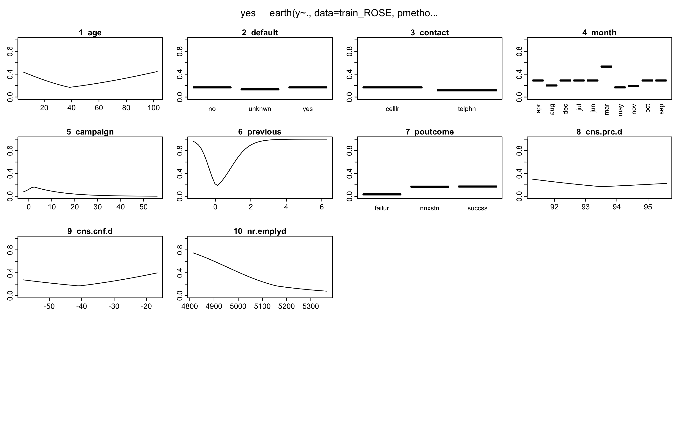
- plotd()함수를 이용해 결과변수 라벨(yes/no)에 따른 예측 확률의 밀도 함수 도표를 볼 수 있다.
> plotd(earth.fit)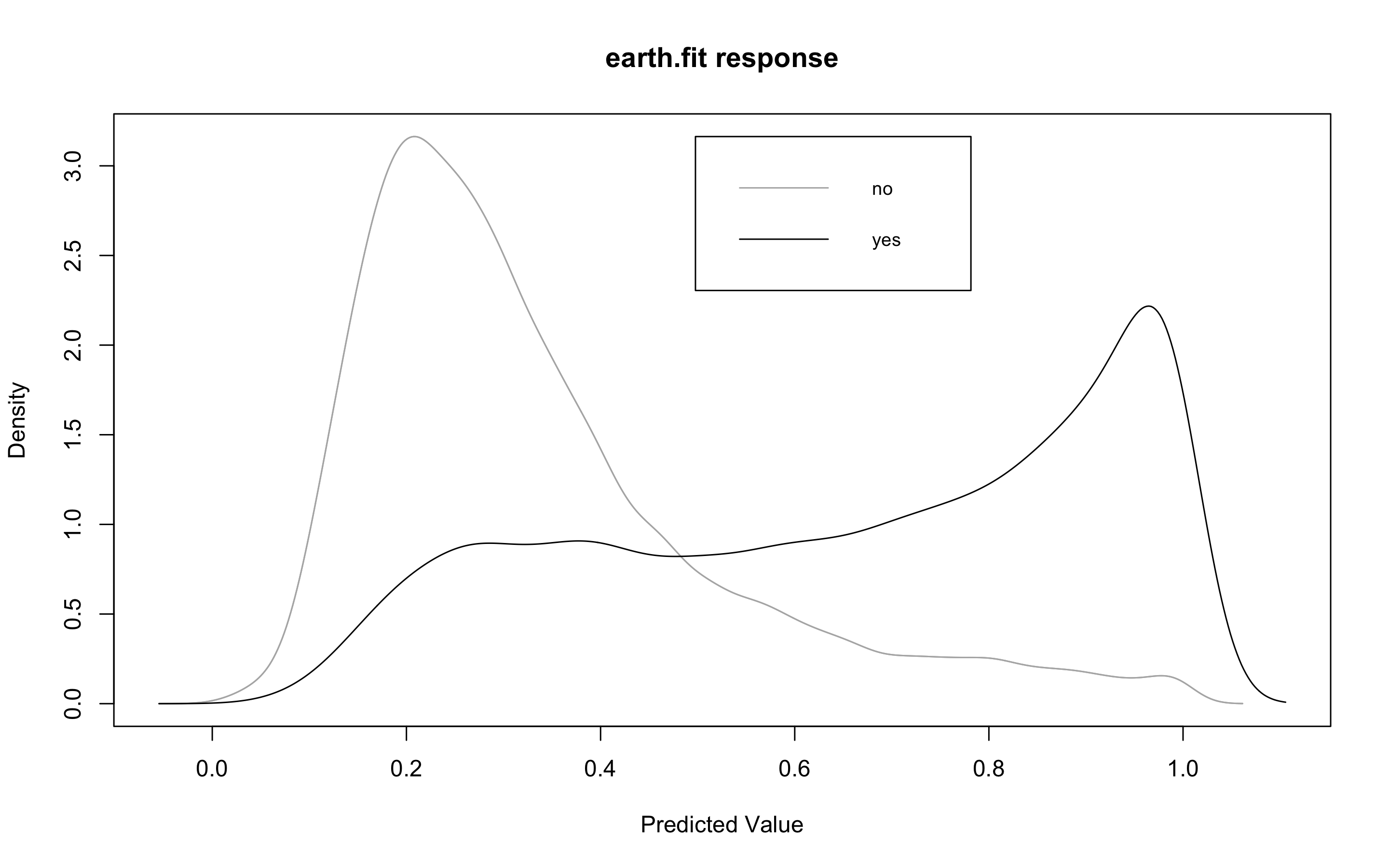
- evimp()함수로 상대적인 변수의 중요도를 살펴보자.
- nsubsets라는 변수명을 볼 수 있는데, 이는 가지치기 패스를 한 후에 남는 변수를 담고 있는 모형의 서브 세트 개수이다.
- gcv와 rss칼럼은 각 예측변수가 기여하는 각 감소값을 나타낸다.
> evimp(earth.fit)
                    nsubsets   gcv    rss
nr.employed               20 100.0  100.0
previous                  19  58.4   58.7
monthmay                  17  44.0   44.5
poutcomesuccess           15  34.5   35.1
cons.price.idx            14  31.5   32.1
monthnov                  13  29.2   29.8
age                       12  26.8   27.4
monthmar                  11  24.8   25.4
campaign                   9  20.6   21.2
poutcomenonexistent        7  16.8   17.4
contacttelephone           6  15.0   15.6
monthaug                   6  15.0   15.6
defaultunknown             4  10.0   10.6
cons.conf.idx 3 6.7 7.4- test데이터에 모형이 얼마나 잘 작동하는지 보자.
> earth.pred <- predict(earth.fit, newdata = test, type = 'response')
> testY <- ifelse(test$y == 'yes', 1, 0)
> library(InformationValue)
> confusionMatrix(testY, earth.pred)
     0   1
0 9584 554
1 1380 838
> misClassError(testY, earth.pred)
[1] 0.1565
> 1 - misClassError(testY, earth.pred)
[1] 0.8435
정확도는 0.8435이다.
- ROC커브를 그려보자
> pred.earth <- prediction(earth.pred, test$y)
> perf.earth <- performance(pred.earth, 'tpr', 'fpr')
> plot(perf.earth, main = 'ROC', col = 1)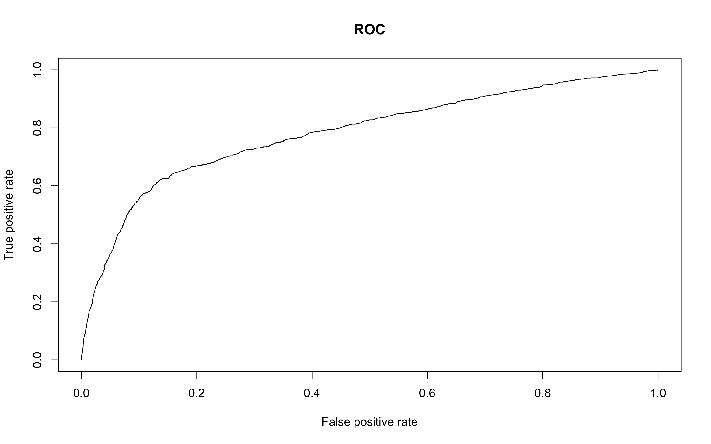
- AUC를 알아보자
> performance(pred.earth, 'auc')@y.values
[[1]]
[1] 0.7837637
MARS 모형의 정확도는 약 84%, AUC는 0.784이다.
KNN
- KNN분석을 해보자.
- KNN은 scale된 데이터와, 예측변수에 팩터형 변수가 있다면 더미변수로 바꿔줘야 한다.
- 위에서 미리 만들어둔 scaled_train_ROSE_dummy데이터와 scaled_test_dummy데이터를 사용하자.
- 먼저 필요한 패키지들을 불러오자
> library(class)
> library(kknn)
> library(e1071)
> library(caret)
> library(MASS)
> library(reshape2)
> library(ggplot2)
> library(kernlab)
> library(ROCR)- KNN을 사용할 때는 가장 적절한 K를 선택하는 일은 매우 중요하다. K를 선택하기 위해 expand.grid()와 seq()함수를 사용해보자.
> knn.train <- train(y ~., data = scaled_train_ROSE_dummy,
+                    method = 'knn',
+                    trControl = control,
+                    tuneGrid = grid1)
> knn.train
k-Nearest Neighbors

28832 samples
   53 predictor
    2 classes: 'no', 'yes'

No pre-processing
Resampling: Cross-Validated (10 fold)
Summary of sample sizes: 25948, 25948, 25949, 25949, 25948, 25949, ...
Resampling results across tuning parameters:

  k   Accuracy   Kappa
   2  0.8354609  0.6708884
   4  0.8343517  0.6686798
   6  0.8204434  0.6407899
   8  0.8106277  0.6210880
  10  0.8009165  0.6015726
  12  0.7930430  0.5857428
  14  0.7871812  0.5739504
  16  0.7817705  0.5630561
  18  0.7760133  0.5514593
  20  0.7735163  0.5464131
  22  0.7700824  0.5394967
  24  0.7651222  0.5295151
  26  0.7623473  0.5239142
  28  0.7615844  0.5223641
  30  0.7595729  0.5183051

Accuracy was used to select the optimal model using the largest value.
The final value used for the model was k = 2.
k매개변수값으로 2가 나왔다. K와 함께 정확도와 카파통계량도 제공하고 있다.
- knn()함수를 이용해보자
> knn.test <- knn(scaled_train_ROSE_dummy[, -54], scaled_test_dummy[, -54], scaled_train_ROSE_dummy[, 54], k = 2)
> detach("package:InformationValue", unload = TRUE)
> confusionMatrix(knn.test, scaled_test_dummy$y, positive = 'yes')
Confusion Matrix and Statistics

          Reference
Prediction   no  yes
       no  8805  626
       yes 2159  766

               Accuracy : 0.7746
                 95% CI : (0.7671, 0.7819)
    No Information Rate : 0.8873
    P-Value [Acc > NIR] : 1

                  Kappa : 0.2386

 Mcnemar's Test P-Value : <2e-16

            Sensitivity : 0.55029
            Specificity : 0.80308
         Pos Pred Value : 0.26188
         Neg Pred Value : 0.93362
             Prevalence : 0.11266
         Detection Rate : 0.06199
   Detection Prevalence : 0.23673
      Balanced Accuracy : 0.67669

       'Positive' Class : yes
정확도는 0.7746 이고 카파통계량은 0.2386이다.
- 성능을 올리기 위해 커널을 입력해보자.
- distance = 2는 절댓값합 거리를 사용함을 의미하고 1은 유클리드 거리를 의미한다.
> kknn.train <- train.kknn(y ~., data = scaled_train_ROSE_dummy,
+                          kmax = 30, distance = 2,
+                          kernel = c('rectangular', 'triangular', 'epanechnikov'))
> plot(kknn.train)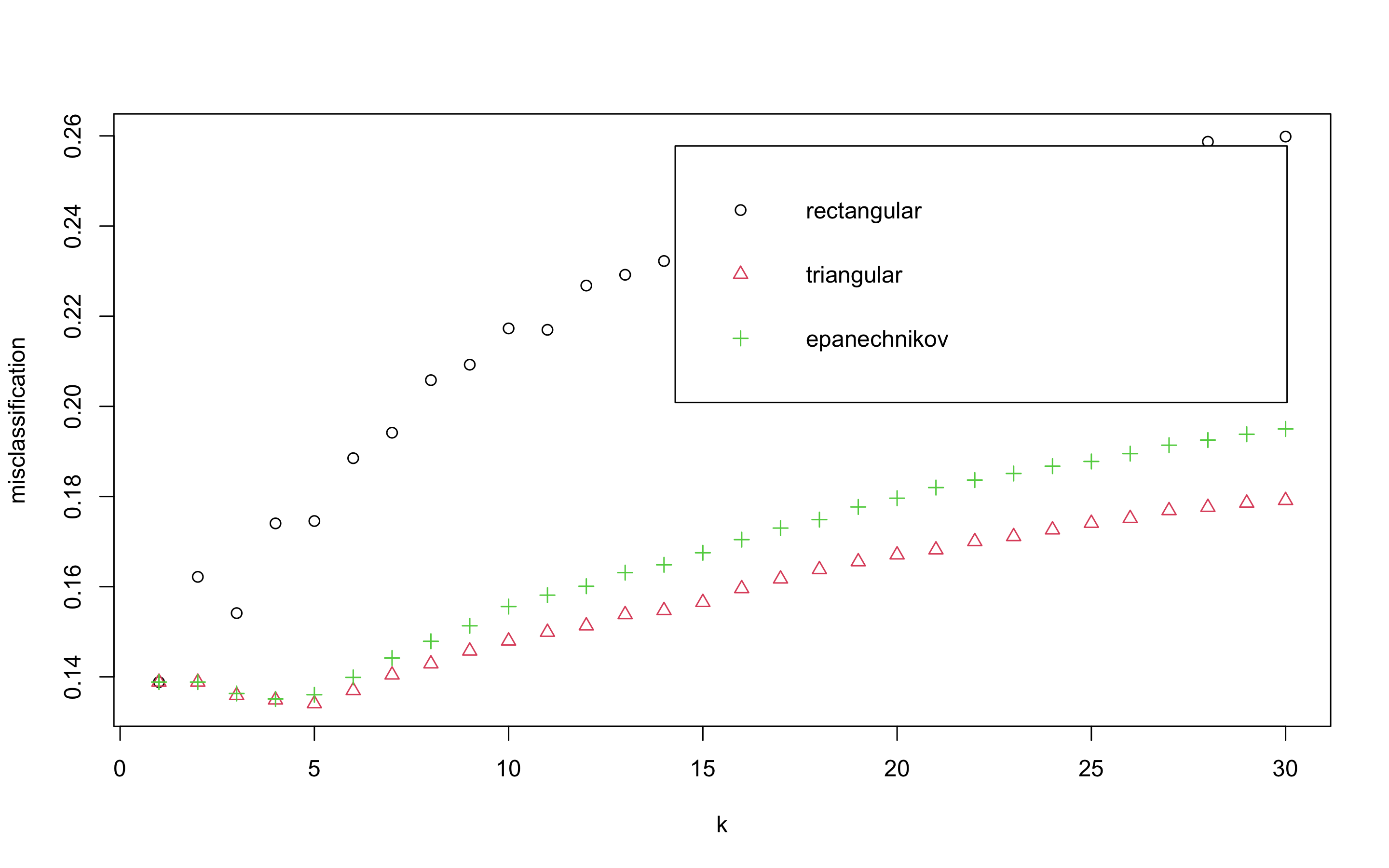
plot은 k값을 x축, 각 커널에 의해 잘못 분류된 관찰값들의 비율을 y축에 표시하고 있다. triangular커널을 사용하고 k = 5일때 가자 오류가 낮은 것으로 보인다.
> kknn.train

Call:
train.kknn(formula = y ~ ., data = scaled_train_ROSE_dummy, kmax = 30,     distance = 2, kernel = c("rectangular", "triangular", "epanechnikov"))

Type of response variable: nominal
Minimal misclassification: 0.1340524
Best kernel: triangular
Best k: 5- 예측 성능을 보자
> kknn.p <- predict(kknn.train, newdata = scaled_test_dummy)
> confusionMatrix(kknn.p, scaled_test_dummy$y, positive = 'yes')
Confusion Matrix and Statistics

          Reference
Prediction   no  yes
       no  8990  681
       yes 1974  711

               Accuracy : 0.7851
                 95% CI : (0.7778, 0.7923)
    No Information Rate : 0.8873
    P-Value [Acc > NIR] : 1

                  Kappa : 0.2353

 Mcnemar's Test P-Value : <2e-16

            Sensitivity : 0.51078
            Specificity : 0.81996
         Pos Pred Value : 0.26480
         Neg Pred Value : 0.92958
             Prevalence : 0.11266
         Detection Rate : 0.05754
   Detection Prevalence : 0.21730
      Balanced Accuracy : 0.66537

       'Positive' Class : yes
정확도는 0.7851, 카파통계량은 0.2353으로 커널이 없을 때(정확도 : 0.7746, 카파통계량 : 0.2386)오히려 성능이 떨어졌다. 따라서 이 데이터로는 훈련시에 거리에 가중값을 주는 방법이 오히려 모형의 정확도를 개선하지 못하고 있다.
- ROC커브를 그리고 AUC를 알아보자
> plot(perf.earth, main = 'ROC', col = 1)
> pred.knn <- prediction(as.numeric(kknn.p), as.numeric(scaled_test_dummy$y))
> perf.knn <- performance(pred.knn, 'tpr', 'fpr')
> plot(perf.knn, col = 2, add = TRUE)
> performance(pred.knn, 'auc')@y.values
[[1]]
[1] 0.665366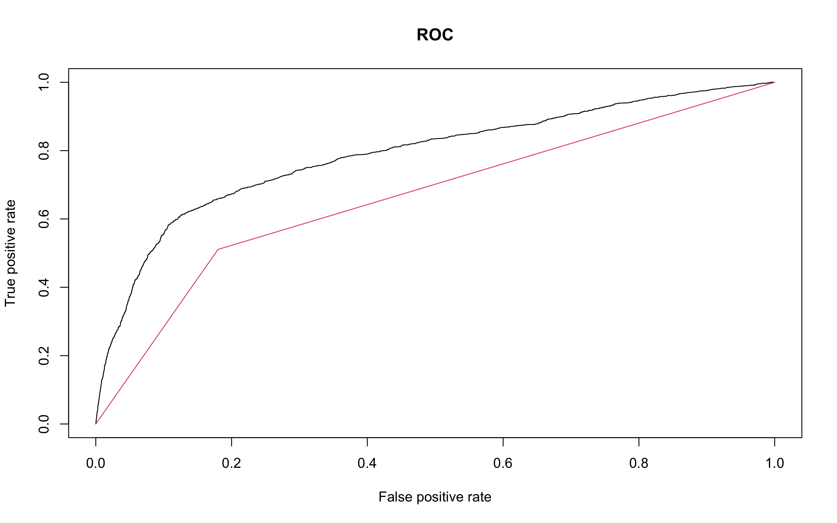
KNN의 AUC는 0.665366로 mars의 auc(0.7837637)보다 낮은 성능을 보인다.
랜덤포레스트
- 다음으로 랜덤포레스트 모델을 만들어 보자.
- train_ROSE, test데이터를 사용한다.
- 필요한 패키지를 부르자.
> library(rpart)
> library(partykit)
> library(MASS)
> library(genridge)
> library(randomForest)
> library(xgboost)
> library(caret)
> library(InformationValue)- 랜덤포레스트 모형을 만들어보자
> set.seed(123)
> rf.model <- randomForest(y ~., data = train_ROSE)
> rf.model

Call:
 randomForest(formula = y ~ ., data = train_ROSE)
               Type of random forest: classification
                     Number of trees: 500
No. of variables tried at each split: 3

        OOB estimate of  error rate: 14.86%
Confusion matrix:
       no   yes class.error
no  12506  2011   0.1385272
yes  2272 12043   0.1587146
수행결과 OOB(out of bag)오차율은 14.86%로 나왔다.
- 개선을 위해 최적의 트리 수를 보자.
> plot(rf.model)
> which.min(rf.model$err.rate[, 1])
[1] 383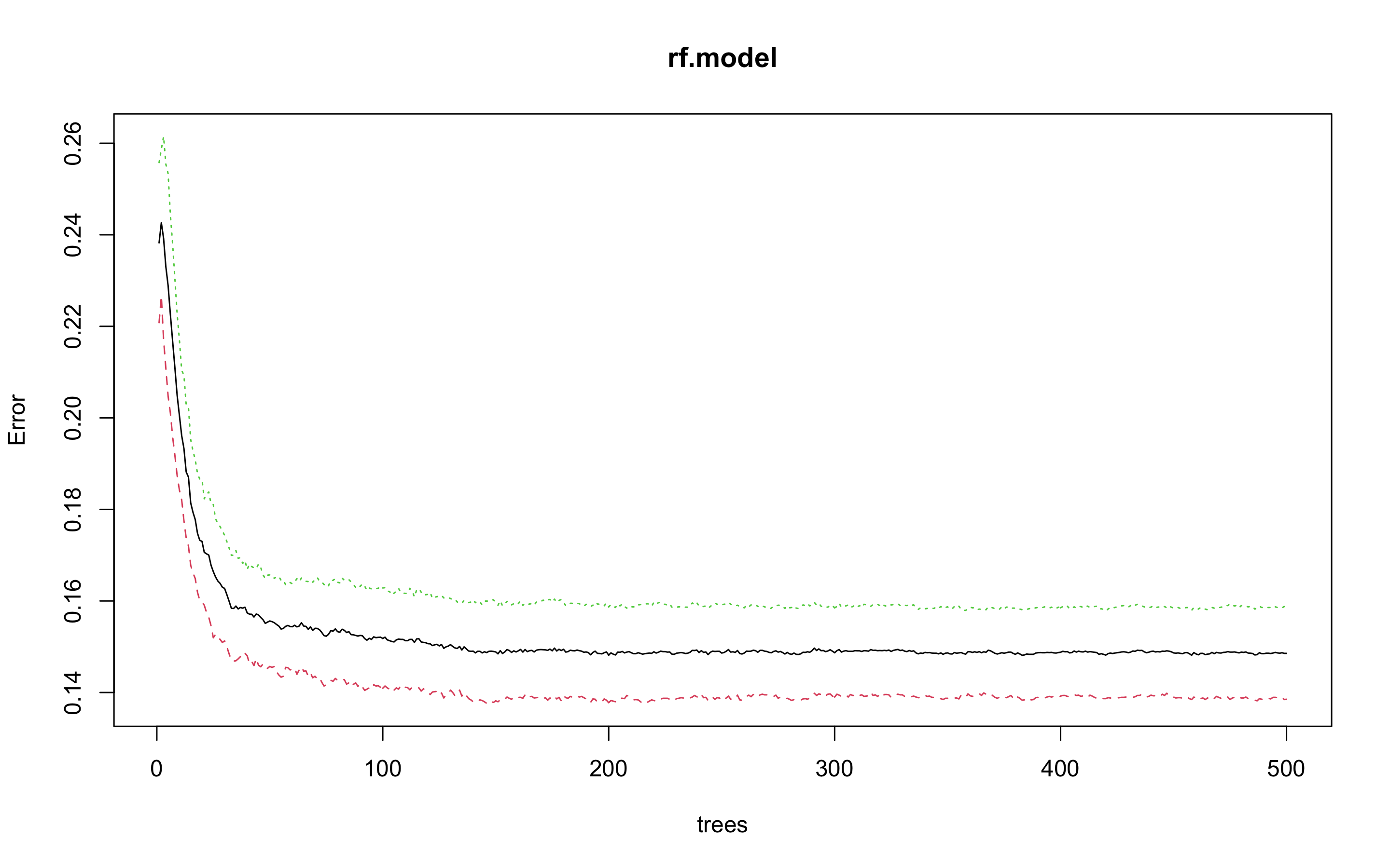
모형 정확도를 최적화 하기에 필요한 트리수가 383개면 된다는 결과를 얻었다.
> set.seed(123)
> rf.model2 <- randomForest(y ~., data = train_ROSE, ntree = 383)
> rf.model2

Call:
 randomForest(formula = y ~ ., data = train_ROSE, ntree = 383)
               Type of random forest: classification
                     Number of trees: 383
No. of variables tried at each split: 3

        OOB estimate of  error rate: 14.81%
Confusion matrix:
       no   yes class.error
no  12509  2008   0.1383206
yes  2263 12052   0.1580859
OOB오차가 14.86%에서 14.81%로 약간 줄어들었다.
- 테스트 데이터로 어떤 결과가 나오는지 보자.
> rf.test <- predict(rf.model2, newdata = test, type = 'response')
> detach("package:InformationValue", unload = TRUE)
> confusionMatrix(rf.test, test$y, positive = 'yes')
Confusion Matrix and Statistics

          Reference
Prediction    no   yes
       no  10240   726
       yes   724   666

               Accuracy : 0.8826
                 95% CI : (0.8768, 0.8883)
    No Information Rate : 0.8873
    P-Value [Acc > NIR] : 0.9514

                  Kappa : 0.4127

 Mcnemar's Test P-Value : 0.9790

            Sensitivity : 0.4784
            Specificity : 0.9340
         Pos Pred Value : 0.4791
         Neg Pred Value : 0.9338
             Prevalence : 0.1127
         Detection Rate : 0.0539
   Detection Prevalence : 0.1125
      Balanced Accuracy : 0.7062

       'Positive' Class : yes
정확도는 0.8826, 카파통계량은 0.4127로 KNN과 earth보다 높은 정확도를 보이고 있다.
- 변수 중요도를 보자
> varImpPlot(rf.model2)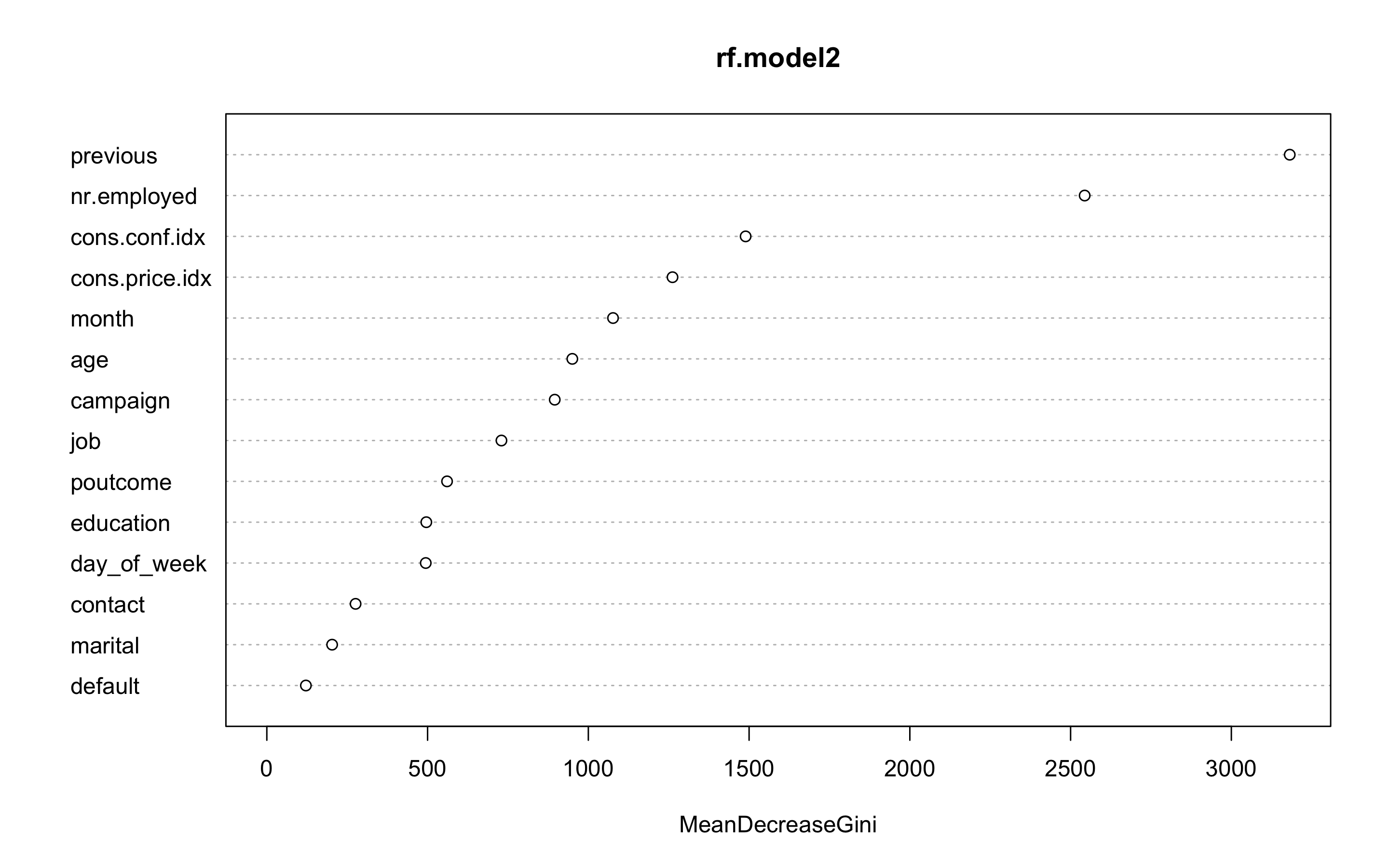
- ROC커브를 그리고 AUC를 알아보자
> pred.rf <- prediction(as.numeric(rf.test), as.numeric(test$y))
> perf.rf <- performance(pred.rf, 'tpr', 'fpr')
> plot(perf.earth, main = 'ROC', col = 1)
> plot(perf.knn, col = 2, add = TRUE)
> plot(perf.rf, col = 3, add = TRUE)
> performance(pred.rf, 'auc')@y.values
[[1]]
[1] 0.706207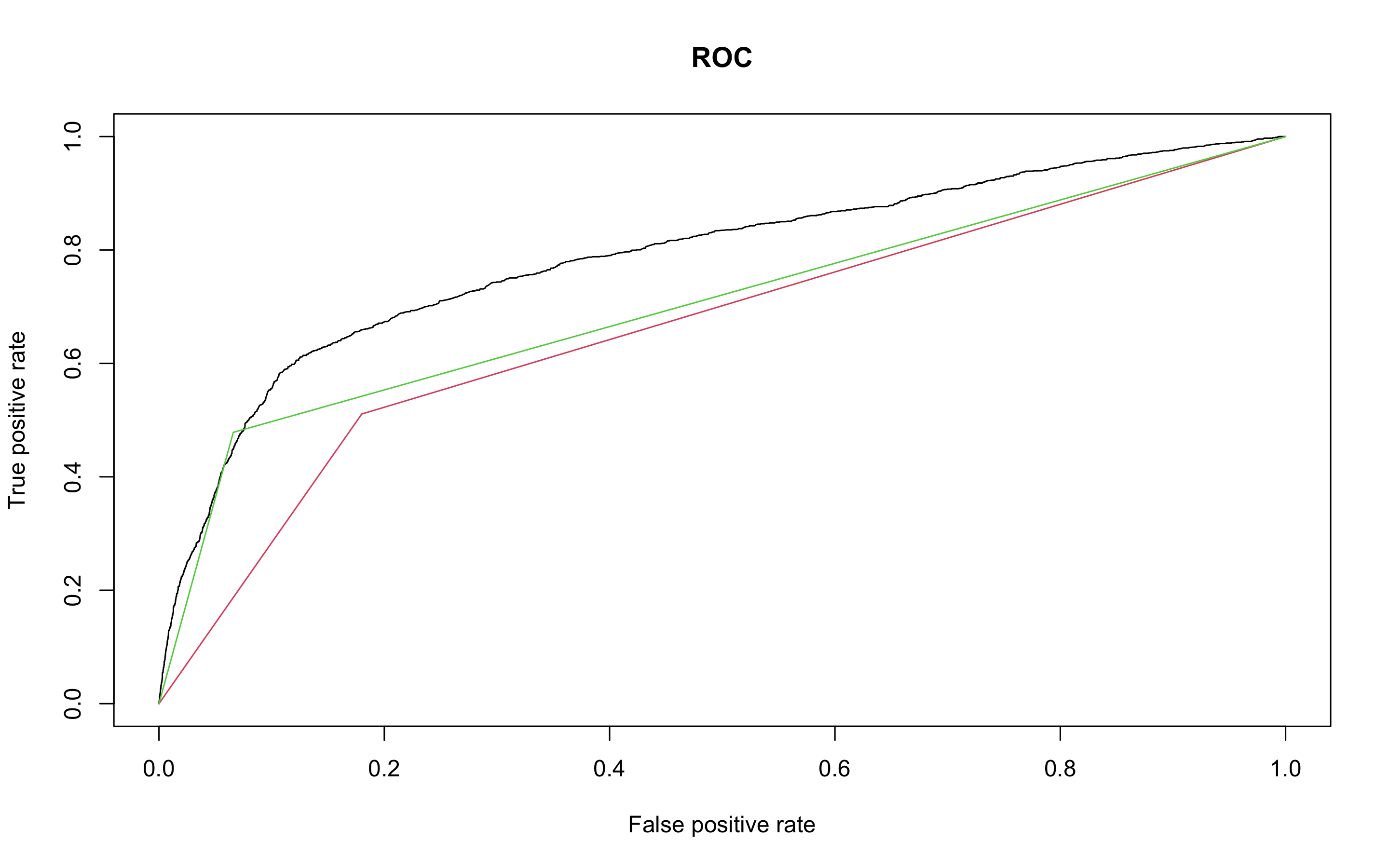
랜덤포레스트의 AUC는 0.706207로 mars보다는 나쁘고 knn보다는 좋은 성능을 보인다.
익스트림 그레디언트 부스트(XGBoost)
- 다음으로 익스트림 그레디언트 부스트 모델을 만들어 보자.
- scaled_train_ROSE_dummy데이터와 scaled_test_dummy데이터를 사용하자.
- 필요한 패키지들을 불러오자.
> library(rpart)
> library(partykit)
> library(MASS)
> library(genridge)
> library(randomForest)
> library(xgboost)
> library(caret)
> library(Boruta)
> library(InformationValue)- 부스트 기법을 사용하기 위해서는 여러 인자값들을 세부 조정해야 한다.
- 그리드를 만들어 보자.
- 각 인자값들은 다음과 같다.
| 인자 | Description |
|---|---|
| nrounds | 최대 반복 횟수(최종 모형에서의 트리 수) |
| colsample_bytree | 트리를 생성할 때 표본 추출할 피처 수(비율로 표시됨), 기본값은 1 |
| min_child_weight | 부스트되는 트리에서 최소 가중값, 기본값은 1 |
| eta | 학습 속도, 해법에 관한 각 트리의 기여도를 의미, 기본값은 0.3 |
| gamma | 트리에서 다른 leaf 분할을 하기 위해 필요한 최소 손실 감소 |
| subsample | 데이터 관찰값의 비율, 기본값은 1 |
| max_depth | 개별 트리의 최대 깊이 |
> grid <- expand.grid(nrounds = c(75, 150),
+                     colsample_bytree = 1,
+                     min_child_weight = 1,
+                     eta = c(0.01, 0.1, 0.3),
+                     gamma = c(0.5, 0.25),
+                     subsample = 0.5,
+                     max_depth = c(2, 3)
+ )- trainControl인자를 조정한다. 여기서는 5-fold교차검증을 사용할 것이다
> cntrl <- trainControl(method = 'cv',
+                       number = 5,
+                       verboseIter = TRUE,
+                       returnData = FALSE,
+ returnResamp = 'final')- train()함수를 사용해 데이터를 학습시킨다.
> set.seed(123)
> train.xgb <- train(x = scaled_train_ROSE_dummy[, 1:53],
                   y = scaled_train_ROSE_dummy[, 54],
                   trControl = cntrl,
                   tuneGrid = grid,
                   method = 'xgbTree')
+ Fold1: eta=0.01, max_depth=2, gamma=0.25, colsample_bytree=1, min_child_weight=1, subsample=0.5, nrounds=150
[21:42:25] WARNING: amalgamation/../src/c_api/c_api.cc:718: `ntree_limit` is deprecated, use `iteration_range` instead.
.
.
.
- Fold5: eta=0.30, max_depth=3, gamma=0.50, colsample_bytree=1, min_child_weight=1, subsample=0.5, nrounds=150
Aggregating results
Selecting tuning parameters
Fitting nrounds = 150, max_depth = 3, eta = 0.3, gamma = 0.5, colsample_bytree = 1, min_child_weight = 1, subsample = 0.5 on full training set
모형을 생성하기 위한 최적 인자들의 조합이 출력되었다.
nrounds = 150, max_depth = 3, eta = 0.3, gamma = 0.5, colsample_bytree = 1, min_child_weight = 1, subsample = 0.5
- xgb.train()에서 사용할 인자 목록을 생성하고, 데이터프레임의 입력피처의 행렬과 숫자레이블을 붙힌 결과 목록으로 변환한다. 그런 다음, 피처와 식별값을 xgb.DMatrix에서 사용할 입력값으로 변환한다
> param <- list(object = 'binary:logistic',
+               booster = 'gbtree',
+               eval_metric = 'error',
+               eta = 0.3,
+               max_depth = 3,
+               subsample = 0.5,
+               colsample_bytree = 1,
+               gamma = 0.5)
> x <- as.matrix(scaled_train_ROSE_dummy[, 1:53])
> y <- ifelse(scaled_train_ROSE_dummy$y == 'yes', 1, 0)
> train.mat <- xgb.DMatrix(data = x, label = y)- 모형을 만들어 보자
> set.seed(123)
> xgb.fit <- xgb.train(params = param, data = train.mat, nrounds = 150)- test데이터에 관한 결과를 보기 전에 변수 중요도를 그려 검토해보자.
- 항목은 gain, cover, frequency 이렇게 세가지를 검사할 수 있다. gain은 피처가 트리에 미치는 정확도의 향상 정도를 나타내는 값, cover는 이 피처와 연관된 전체 관찰값의 상대 수치, frequency는 모든 트리에 관해 피처가 나타난 횟수를 백분율로 나타낸 값이다.
> impMatrix <- xgb.importance(feature_names = dimnames(x)[[2]], model = xgb.fit)
> impMatrix
                          Feature         Gain        Cover   Frequency
 1:                   nr.employed 0.3727003954 0.1776517308 0.173869347
 2:                      previous 0.2959397494 0.1200752357 0.138693467
 3:                 cons.conf.idx 0.0724553757 0.1442906677 0.145728643
 4:                     month.may 0.0634221502 0.0110257352 0.017085427
 5:                cons.price.idx 0.0413852543 0.1461441650 0.124623116
 6:                           age 0.0311042003 0.1393180427 0.107537688
 7:                      campaign 0.0264173720 0.0895831339 0.085427136
 8:              poutcome.failure 0.0238098131 0.0073000055 0.012060302
 9:              poutcome.success 0.0121387931 0.0043134393 0.010050251
10:                     month.apr 0.0093261284 0.0064180475 0.013065327
11:              contact.cellular 0.0086068861 0.0147410740 0.015075377
12:                     month.nov 0.0047142423 0.0077213050 0.009045226
13:                     month.oct 0.0038791447 0.0041889072 0.005025126
14:                     month.jul 0.0027124555 0.0064040357 0.009045226
15:                     month.jun 0.0022066649 0.0059288930 0.007035176
16:                     month.aug 0.0021161629 0.0061017580 0.006030151
17:               job.blue-collar 0.0020466868 0.0060845974 0.007035176
18:            education.basic.6y 0.0014927794 0.0088302862 0.008040201
19:                    default.no 0.0014168774 0.0054088809 0.005025126
20:               day_of_week.mon 0.0013496951 0.0041843415 0.004020101
21:               day_of_week.thu 0.0012970639 0.0049945086 0.006030151
22:          poutcome.nonexistent 0.0012685747 0.0026624050 0.003015075
23:                job.technician 0.0011813677 0.0034736741 0.006030151
24:               day_of_week.fri 0.0011164718 0.0036655890 0.005025126
25:         education.high.school 0.0009906457 0.0047914158 0.004020101
26:            education.basic.9y 0.0009760985 0.0012851524 0.004020101
27:               day_of_week.wed 0.0009534717 0.0070666850 0.005025126
28:                     month.mar 0.0009419463 0.0060005265 0.004020101
29:                  job.services 0.0008696435 0.0027940217 0.004020101
30:              job.entrepreneur 0.0008258651 0.0028551070 0.004020101
31:               day_of_week.tue 0.0008087148 0.0002413498 0.004020101
32:   education.university.degree 0.0007867720 0.0015562577 0.002010050
33:                    job.admin. 0.0007845404 0.0036613382 0.004020101
34:             job.self-employed 0.0007793958 0.0005875522 0.004020101
35:                job.management 0.0007467099 0.0015658613 0.004020101
36:                   job.student 0.0007272317 0.0024394752 0.004020101
37:                   job.retired 0.0007084400 0.0010630098 0.003015075
38:                     month.dec 0.0006756035 0.0030451326 0.003015075
39:                 job.housemaid 0.0006626302 0.0066768727 0.004020101
40:                marital.single 0.0006615550 0.0047813399 0.003015075
41:            education.basic.4y 0.0005783666 0.0063799479 0.003015075
42:               marital.married 0.0005748683 0.0003858763 0.003015075
43:                     month.sep 0.0005742491 0.0016463112 0.002010050
44: education.professional.course 0.0003359835 0.0031088943 0.002010050
45:                   job.unknown 0.0002969791 0.0002964525 0.002010050
46:                job.unemployed 0.0002647336 0.0038779705 0.002010050
47:             education.unknown 0.0001983844 0.0010881996 0.001005025
48:              marital.divorced 0.0001728660 0.0022947913 0.001005025
                          Feature         Gain        Cover   Frequency
> xgb.plot.importance(impMatrix, main = 'Gain by Feature')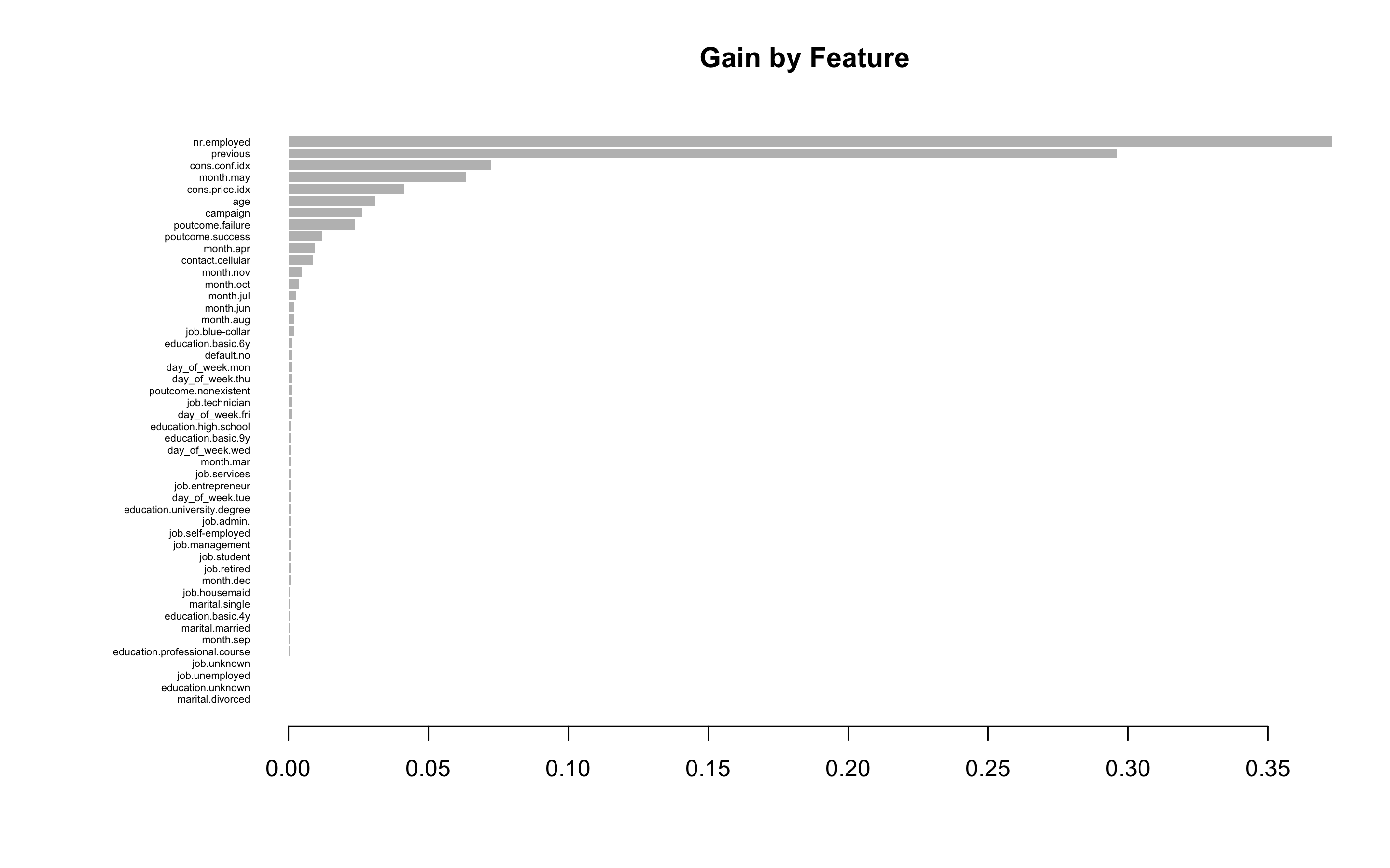
- scaled_test_dummy세트에 관한 수행 결과를 보자
> testMat <- as.matrix(scaled_test_dummy[, 1:53])
> xgb.test <- predict(xgb.fit, testMat)
> y.test <- ifelse(scaled_test_dummy$y == 'yes', 1, 0)
> library(InformationValue)
> detach("package:caret", unload = TRUE)
> confusionMatrix(y.test, xgb.test, threshold = 0.4764343)
     0   1
0 8898 487
1 2066 905
> 1 - misClassError(y.test, xgb.test, threshold = 0.4764343)
[1] 0.7934
정확도는 0.7934다.
- ROC커브를 그려보자
> plotROC(y.test, xgb.test)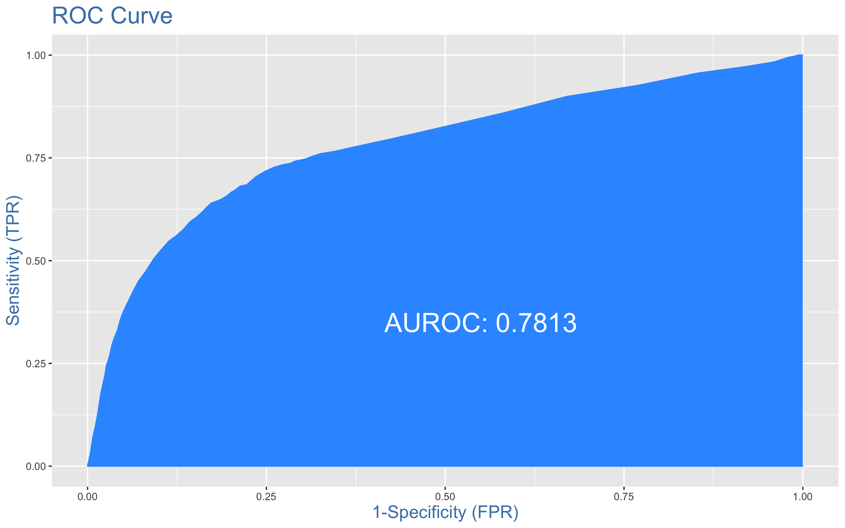
XGBoost의 정확도는 0.7934, AUC는 0.7813이다.
MARS 모형의 AUC는 0.784와 거의 비슷한 성능을 보이고 있다.
사용한 패키지
DMwR2, pastecs, psych, caret, ggplot2, GGally, smotefamily, naniar, reshape2, gridExtra, gapminder, dplyr, PerformanceAnalytics, FSelector, Boruta, ROSE, MASS, bestglm, earth, ROCR, car, corrplot, InformationValue, class, kknn, e1071, kernlab, rpart, partykit, genridge, randomForest, xgboost

2개의 댓글

Bank marketing data sets provide valuable insights into customer behaviors and trends. If you're looking to streamline your financial data, converting bank statements to CSV format can make a huge difference. Using tools like https://www.supaclerk.com/, you can easily convert your bank statements into CSV for better organization and analysis.
Bank marketing data sets provide valuable insights into customer behaviors and trends. If you're looking to streamline your financial data, converting bank statements to CSV format can make a huge difference. Using tools like https://www.supaclerk.com/, you can easily convert your bank statements into CSV for better organization and analysis.