Body Performance Data
데이터 출처
This is data that confirmed the grade of performance with age and some exercise performance data.
데이터는 총 12개의 칼럼과 13393개의 rows로 구성
| Header | Description |
|---|---|
| age | 20 ~64 |
| gender | F,M |
| height_cm | - |
| weight_kg | - |
| body fat_% | - |
| diastolic | diastolic blood pressure (min) |
| systolic | systolic blood pressure (min) |
| gripForce | - |
| sit and bend forward_cm | - |
| sit-ups counts | - |
| broad jump_cm | - |
| class | A,B,C,D ( A: best) / stratified |
EDA
- 데이터 구조 파악
> df <- read.csv(file = 'bodyPerformance.csv', stringsAsFactors = TRUE)
> head(df)
  age gender height_cm weight_kg body.fat_. diastolic systolic gripForce sit.and.bend.forward_cm sit.ups.counts
1  27      M       172      75.2       21.3        80      130      54.9                    18.4             60
2  25      M       165      55.8       15.7        77      126      36.4                    16.3             53
3  31      M       180      78.0       20.1        92      152      44.8                    12.0             49
4  32      M       174      71.1       18.4        76      147      41.4                    15.2             53
5  28      M       174      67.7       17.1        70      127      43.5                    27.1             45
6  36      F       165      55.4       22.0        64      119      23.8                    21.0             27
  broad.jump_cm class
1           217     C
2           229     A
3           181     C
4           219     B
5           217     B
6           153     B
> str(df)
'data.frame':	13393 obs. of  12 variables:
 $ age                    : num  27 25 31 32 28 36 42 33 54 28 ...
 $ gender                 : Factor w/ 2 levels "F","M": 2 2 2 2 2 1 1 2 2 2 ...
 $ height_cm              : num  172 165 180 174 174 ...
 $ weight_kg              : num  75.2 55.8 78 71.1 67.7 ...
 $ body.fat_.             : num  21.3 15.7 20.1 18.4 17.1 22 32.2 36.9 27.6 14.4 ...
 $ diastolic              : num  80 77 92 76 70 64 72 84 85 81 ...
 $ systolic               : num  130 126 152 147 127 119 135 137 165 156 ...
 $ gripForce              : num  54.9 36.4 44.8 41.4 43.5 23.8 22.7 45.9 40.4 57.9 ...
 $ sit.and.bend.forward_cm: num  18.4 16.3 12 15.2 27.1 21 0.8 12.3 18.6 12.1 ...
 $ sit.ups.counts         : num  60 53 49 53 45 27 18 42 34 55 ...
 $ broad.jump_cm          : num  217 229 181 219 217 153 146 234 148 213 ...
 $ class                  : Factor w/ 4 levels "A","B","C","D": 3 1 3 2 2 2 4 2 3 2 ...
> dim(df)
[1] 13393    12
> summary(df)
      age       gender     height_cm     weight_kg       body.fat_.     diastolic        systolic     gripForce
 Min.   :21.0   F:4926   Min.   :125   Min.   : 26.3   Min.   : 3.0   Min.   :  0.0   Min.   :  0   Min.   : 0.0
 1st Qu.:25.0   M:8467   1st Qu.:162   1st Qu.: 58.2   1st Qu.:18.0   1st Qu.: 71.0   1st Qu.:120   1st Qu.:27.5
 Median :32.0            Median :169   Median : 67.4   Median :22.8   Median : 79.0   Median :130   Median :37.9
 Mean   :36.8            Mean   :169   Mean   : 67.4   Mean   :23.2   Mean   : 78.8   Mean   :130   Mean   :37.0
 3rd Qu.:48.0            3rd Qu.:175   3rd Qu.: 75.3   3rd Qu.:28.0   3rd Qu.: 86.0   3rd Qu.:141   3rd Qu.:45.2
 Max.   :64.0            Max.   :194   Max.   :138.1   Max.   :78.4   Max.   :156.2   Max.   :201   Max.   :70.5
 sit.and.bend.forward_cm sit.ups.counts broad.jump_cm class
 Min.   :-25.0           Min.   : 0.0   Min.   :  0   A:3348
 1st Qu.: 10.9           1st Qu.:30.0   1st Qu.:162   B:3347
 Median : 16.2           Median :41.0   Median :193   C:3349
 Mean   : 15.2           Mean   :39.8   Mean   :190   D:3349
 3rd Qu.: 20.7           3rd Qu.:50.0   3rd Qu.:221
 Max.   :213.0           Max.   :80.0   Max.   :303
결측값은 없으며, summary(df)를 보았을 때 sit.and.bend.forward_cm변수와 broad.jump_cm변수에 이상치가 있는 것으로 보인다.
- 탐색적 분석으로 첨도 및 왜도를 확인해보자
> library(pastecs)
> library(psych)
> describeBy(df[, -c(2, 12)], df$class, mat = FALSE)

 Descriptive statistics by group
group: A
                        vars    n  mean    sd median trimmed   mad   min   max range  skew kurtosis   se
age                        1 3348  35.3 13.00   30.0    33.8 10.38  21.0  64.0  43.0  0.86    -0.56 0.22
height_cm                  2 3348 167.9  7.84  168.0   167.9  8.90 140.5 191.8  51.3 -0.03    -0.53 0.14
weight_kg                  3 3348  64.4 10.55   64.5    64.2 12.25  34.5 101.4  66.9  0.20    -0.56 0.18
body.fat_.                 4 3348  20.5  6.44   20.2    20.4  6.82   3.0  78.4  75.4  0.42     1.33 0.11
diastolic                  5 3348  77.9 10.60   78.0    78.0 11.12  41.0 126.0  85.0 -0.05    -0.19 0.18
systolic                   6 3348 129.3 14.77  128.0   129.1 14.83  14.0 201.0 187.0  0.04     0.88 0.26
gripForce                  7 3348  38.6 10.89   39.0    38.3 14.31   2.1  70.5  68.4  0.13    -1.06 0.19
sit.and.bend.forward_cm    8 3348  21.4  5.12   21.1    21.2  4.37  11.8 185.0 173.2  9.90   308.84 0.09
sit.ups.counts             9 3348  47.9 10.82   49.0    48.2 11.86  17.0  80.0  63.0 -0.31    -0.25 0.19
broad.jump_cm             10 3348 202.7 35.89  202.0   203.3 44.48  40.0 299.0 259.0 -0.13    -0.73 0.62
---------------------------------------------------------------------------------------
group: B
                        vars    n  mean    sd median trimmed   mad   min   max range  skew kurtosis   se
age                        1 3347  37.1 13.70   32.0    36.0 13.34  21.0  64.0  43.0  0.59    -1.05 0.24
height_cm                  2 3347 168.6  8.13  169.2   168.8  8.45 125.0 191.8  66.8 -0.23    -0.22 0.14
weight_kg                  3 3347  66.6 10.88   67.1    66.5 11.71  31.9 111.8  79.9  0.11    -0.37 0.19
body.fat_.                 4 3347  22.0  6.65   21.7    21.9  6.97   4.7  44.5  39.8  0.23    -0.43 0.11
diastolic                  5 3347  78.7 10.66   79.0    78.8 10.38   6.0 112.0 106.0 -0.28     0.74 0.18
systolic                   6 3347 130.6 14.48  130.0   130.6 14.83  43.9 193.0 149.1 -0.02    -0.02 0.25
gripForce                  7 3347  37.9 10.39   39.6    37.9 12.31   0.0  69.9  69.9 -0.05    -0.85 0.18
sit.and.bend.forward_cm    8 3347  17.5  5.91   17.0    17.2  4.89   7.1 213.0 205.9 11.08   357.09 0.10
sit.ups.counts             9 3347  42.6 11.74   44.0    43.0 13.34  12.0  78.0  66.0 -0.28    -0.50 0.20
broad.jump_cm             10 3347 195.3 36.31  200.0   196.6 41.51  71.0 295.0 224.0 -0.27    -0.64 0.63
---------------------------------------------------------------------------------------
group: C
                        vars    n  mean    sd median trimmed   mad   min   max range  skew kurtosis   se
age                        1 3349  36.7 13.78   32.0    35.5 13.34  21.0  64.0  43.0  0.58    -1.05 0.24
height_cm                  2 3349 169.2  8.52  170.0   169.4  8.75 141.0 193.8  52.8 -0.28    -0.43 0.15
weight_kg                  3 3349  66.8 10.86   67.2    66.7 11.71  38.1 103.6  65.5  0.06    -0.52 0.19
body.fat_.                 4 3349  22.6  6.27   22.2    22.5  5.78   3.5  43.0  39.5  0.26    -0.20 0.11
diastolic                  5 3349  78.5 10.64   79.0    78.7 10.38  40.0 156.2 116.2 -0.03     0.52 0.18
systolic                   6 3349 129.9 14.52  130.0   129.9 14.83  91.0 195.0 104.0  0.05    -0.38 0.25
gripForce                  7 3349  36.6 10.22   38.0    36.5 12.01   0.0  65.2  65.2 -0.05    -0.89 0.18
sit.and.bend.forward_cm    8 3349  14.4  5.88   14.0    14.1  6.52   2.3  37.0  34.7  0.43    -0.24 0.10
sit.ups.counts             9 3349  38.7 12.73   40.0    39.1 13.34   7.0  71.0  64.0 -0.25    -0.60 0.22
broad.jump_cm             10 3349 188.6 39.36  194.0   190.4 43.00   0.0 303.0 303.0 -0.44    -0.07 0.68
---------------------------------------------------------------------------------------
group: D
                        vars    n   mean    sd median trimmed   mad   min   max range  skew kurtosis   se
age                        1 3349  38.06 13.86   36.0   37.18 17.79  21.0  64.0  43.0  0.39    -1.23 0.24
height_cm                  2 3349 168.63  9.11  169.7  168.84  9.93 139.5 192.0  52.5 -0.22    -0.56 0.16
weight_kg                  3 3349  72.00 13.88   71.8   71.63 14.68  26.3 138.1 111.8  0.30     0.09 0.24
body.fat_.                 4 3349  27.74  7.51   27.4   27.67  7.56   3.5  54.9  51.4  0.10    -0.11 0.13
diastolic                  5 3349  80.08 10.96   80.0   80.33 11.86   0.0 120.0 120.0 -0.31     0.48 0.19
systolic                   6 3349 131.08 15.02  131.0  131.28 16.31   0.0 181.0 181.0 -0.26     0.97 0.26
gripForce                  7 3349  34.75 10.58   35.6   34.69 12.60   0.0  70.4  70.4  0.00    -0.70 0.18
sit.and.bend.forward_cm    8 3349   7.59  9.39    7.7    7.89  9.64 -25.0  35.2  60.2 -0.28    -0.19 0.16
sit.ups.counts             9 3349  29.88 15.03   30.0   30.19 16.31   0.0  78.0  78.0 -0.14    -0.62 0.26
broad.jump_cm             10 3349 173.82 41.82  180.0  175.76 44.48   0.0 275.0 275.0 -0.48     0.01 0.72
각 class별 평균을 보았을 때 A그룹에 비해 D그룹의 몸무게가 각각 64, 72kg으로 꽤 차이나는 것으로 보인다. 또한 대부분의 변수는 첨도와 왜도가 0에 가까워 표준정규분포를 따르는 것처럼 보이지만 sit.and.bend.forward_cm 변수는 A그룹에서 왜도 9.9, 첨도 308.84로 정규분포에서 크게 벗어나 있는 것으로 보인다.
- 변수들의 상관관계를 확인해보자
> df_numeric <- df[, -c(2, 12)]
> cor_df <- cor(df_numeric)
> cor_df
                           age height_cm weight_kg body.fat_. diastolic systolic gripForce sit.and.bend.forward_cm
age                      1.000    -0.294   -0.1000     0.2423    0.1585   0.2112    -0.180                 -0.0700
height_cm               -0.294     1.000    0.7349    -0.5154    0.1459   0.2102     0.735                 -0.2220
weight_kg               -0.100     0.735    1.0000    -0.0841    0.2623   0.3389     0.700                 -0.2962
body.fat_.               0.242    -0.515   -0.0841     1.0000    0.0481  -0.0304    -0.542                 -0.0712
diastolic                0.159     0.146    0.2623     0.0481    1.0000   0.6763     0.202                 -0.0721
systolic                 0.211     0.210    0.3389    -0.0304    0.6763   1.0000     0.286                 -0.0824
gripForce               -0.180     0.735    0.7001    -0.5418    0.2021   0.2860     1.000                 -0.1126
sit.and.bend.forward_cm -0.070    -0.222   -0.2962    -0.0712   -0.0721  -0.0824    -0.113                  1.0000
sit.ups.counts          -0.545     0.500    0.2949    -0.6089    0.0165   0.0563     0.577                  0.1772
broad.jump_cm           -0.435     0.675    0.4796    -0.6733    0.0972   0.1529     0.747                  0.0265
                        sit.ups.counts broad.jump_cm
age                            -0.5446       -0.4352
height_cm                       0.5004        0.6746
weight_kg                       0.2949        0.4796
body.fat_.                     -0.6089       -0.6733
diastolic                       0.0165        0.0972
systolic                        0.0563        0.1529
gripForce                       0.5767        0.7469
sit.and.bend.forward_cm         0.1772        0.0265
sit.ups.counts                  1.0000        0.7483
broad.jump_cm                   0.7483        1.0000
> library(PerformanceAnalytics)
> chart.Correlation(df_numeric, histogram = TRUE, pch = 19, method = 'pearson')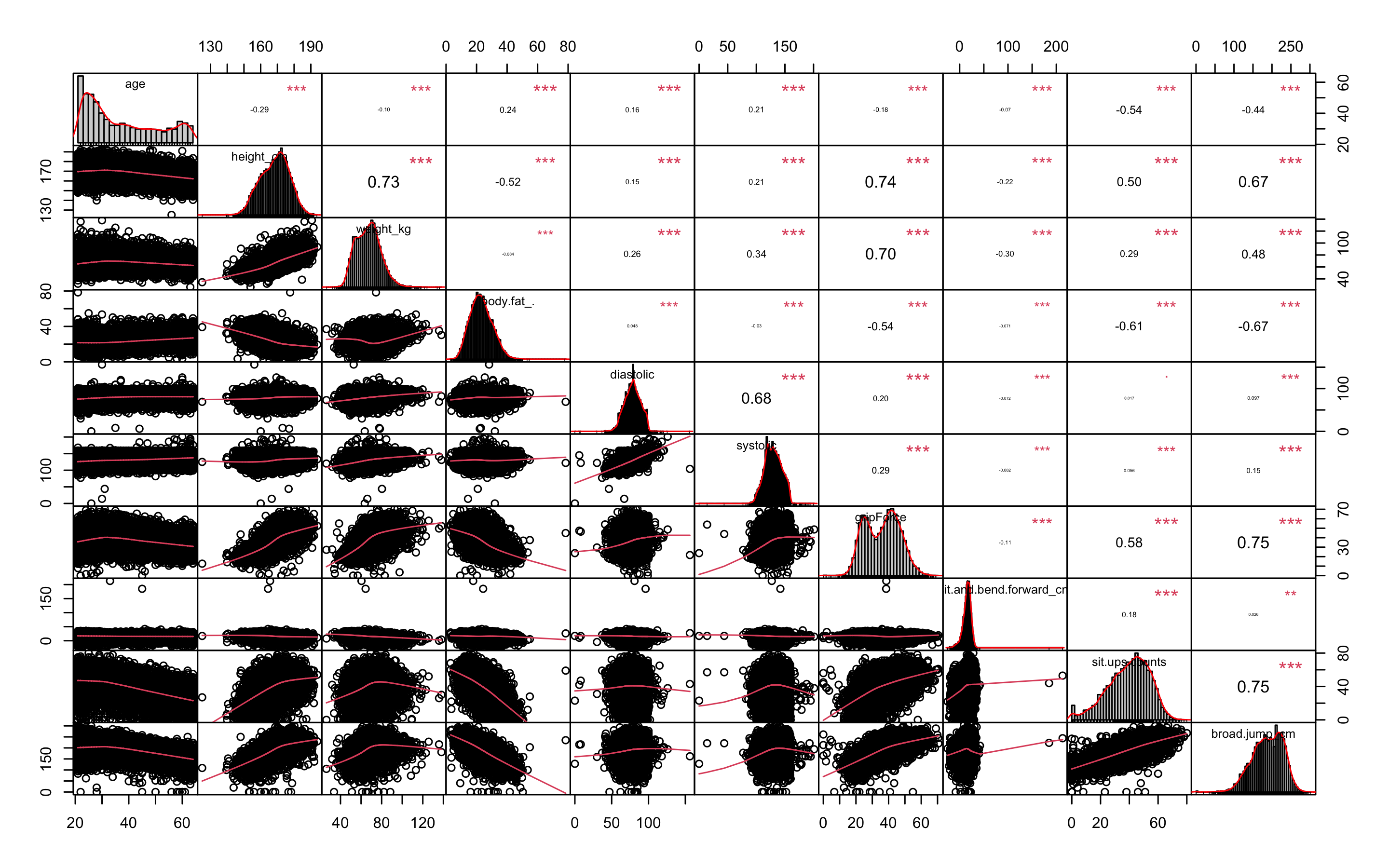
상관관계가 0.8이 넘는 변수는 존재하지 않지만, 0.74를 넘는 상관관계를 가진 변수를 제거해보자
- 상관관계가 0.74 초과인 변수를 찾아내고 제거해준다.
> library(caret)
> findCorrelation(cor_df, cutoff = 0.74)
[1]  7 10
> str(df_numeric)
'data.frame':	13393 obs. of  10 variables:
 $ age                    : num  27 25 31 32 28 36 42 33 54 28 ...
 $ height_cm              : num  172 165 180 174 174 ...
 $ weight_kg              : num  75.2 55.8 78 71.1 67.7 ...
 $ body.fat_.             : num  21.3 15.7 20.1 18.4 17.1 22 32.2 36.9 27.6 14.4 ...
 $ diastolic              : num  80 77 92 76 70 64 72 84 85 81 ...
 $ systolic               : num  130 126 152 147 127 119 135 137 165 156 ...
 $ gripForce              : num  54.9 36.4 44.8 41.4 43.5 23.8 22.7 45.9 40.4 57.9 ...
 $ sit.and.bend.forward_cm: num  18.4 16.3 12 15.2 27.1 21 0.8 12.3 18.6 12.1 ...
 $ sit.ups.counts         : num  60 53 49 53 45 27 18 42 34 55 ...
 $ broad.jump_cm          : num  217 229 181 219 217 153 146 234 148 213 ...
 > df_numeric_2 <- df_numeric[, -c(7, 10)]
> str(df_numeric_2)
'data.frame':	13393 obs. of  8 variables:
 $ age                    : num  27 25 31 32 28 36 42 33 54 28 ...
 $ height_cm              : num  172 165 180 174 174 ...
 $ weight_kg              : num  75.2 55.8 78 71.1 67.7 ...
 $ body.fat_.             : num  21.3 15.7 20.1 18.4 17.1 22 32.2 36.9 27.6 14.4 ...
 $ diastolic              : num  80 77 92 76 70 64 72 84 85 81 ...
 $ systolic               : num  130 126 152 147 127 119 135 137 165 156 ...
 $ sit.and.bend.forward_cm: num  18.4 16.3 12 15.2 27.1 21 0.8 12.3 18.6 12.1 ...
$ sit.ups.counts : num 60 53 49 53 45 27 18 42 34 55 ...- 분산이 0에 가까운 변수도 제거한다.
'변수를 선택하는 기법 중 가장 단순한 방법은 변숫값의 분산을 보는 것이다. 예를 들어, 데이터 1000개가 있는데 이 중 990개는 변수 A의 값이 0, 10개에서 변수 A의 값이 1이라고 하자. 그러면 변수 A는 서로 다른 관찰을 구별하는 데 별 소용이 없다. 따라서 데이터 모델링에서도 그리 유용하지 않다. 이런 변수는 분산이 0에 가까우므로 분석 전에 제거해준다.
> nearZeroVar(df_numeric_2, saveMetrics = TRUE)
                        freqRatio percentUnique zeroVar   nzv
age                      1.221800     0.3285298   FALSE FALSE
height_cm                1.125000     3.4868961   FALSE FALSE
weight_kg                1.039216    10.4382887   FALSE FALSE
body.fat_.               1.034483     3.9348914   FALSE FALSE
diastolic                1.390041     0.6645262   FALSE FALSE
systolic                 1.237981     0.7615919   FALSE FALSE
sit.and.bend.forward_cm  1.166667     3.9423579   FALSE FALSE
sit.ups.counts           1.055838     0.6047935   FALSE FALSE
분산이 0에 가까운 변수는 없다!(분산이 0에 가까운 변수는 위 출력의 nzv부분이 TRUE로 나온다)
- 팩터형 변수들을 데이터 프레임에 다시 합친다.
> df_numeric_2$gender <- df$gender
> df_numeric_2$class <- df$class
> str(df_numeric_2)
'data.frame':	13393 obs. of  10 variables:
 $ age                    : num  27 25 31 32 28 36 42 33 54 28 ...
 $ height_cm              : num  172 165 180 174 174 ...
 $ weight_kg              : num  75.2 55.8 78 71.1 67.7 ...
 $ body.fat_.             : num  21.3 15.7 20.1 18.4 17.1 22 32.2 36.9 27.6 14.4 ...
 $ diastolic              : num  80 77 92 76 70 64 72 84 85 81 ...
 $ systolic               : num  130 126 152 147 127 119 135 137 165 156 ...
 $ sit.and.bend.forward_cm: num  18.4 16.3 12 15.2 27.1 21 0.8 12.3 18.6 12.1 ...
 $ sit.ups.counts         : num  60 53 49 53 45 27 18 42 34 55 ...
 $ gender                 : Factor w/ 2 levels "F","M": 2 2 2 2 2 1 1 2 2 2 ...
 $ class                  : Factor w/ 4 levels "A","B","C","D": 3 1 3 2 2 2 4 2 3 2 ...
결과변수인 class를 제외한 설명변수가 9개로 적당해 보인다.
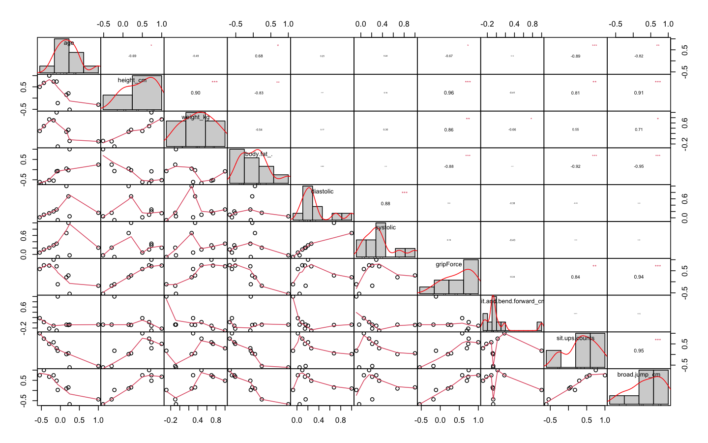
- GGally패키지의 ggpairs함수를 통해 전체적인 그래프를 확인해보자.
> library(GGally)
> ggpairs(df_numeric_2, aes(colour = class))
class별로 다른 색으로 그래프를 보여준다. 맨 오른쪽의 class줄을 보면 boxplot의 범위를 벗어나는 이상치가 보인다. 위의 첨도 왜도 분석에서 보았듯이 sit.and.bend.forward_cm변수의 히스토그램은 왼쪽으로 쏠려있고 뾰족한 것으로 보인다.
또 하나를 말하자면 그래프가 나오는데 꽤 오랜 시간이 걸린다. 변수가 많다면 ggpairs로 그래프 그리는 것을 시도하지 않는 편이 좋다.
- ggpairs가 복잡해서 보기 힘들다면 따로 boxplot을 그려보자.
- 원래 데이터의 범위가 변수별로 차이나므로 평균이 0, 분산이 1이 되도록 스케일링 해주고, 데이터를 wide형식에서 long형식으로 바꿔준다.
> library(reshape2)
> model_scale <- preProcess(df_numeric_2, method = c('center', 'scale'))
> scaled_df <- predict(model_scale, df_numeric_2)
> scaled_df_2 <- scaled_df[, -9]
> melt_df <- melt(scaled_df_2, id.vars = 'class')
> head(melt_df)
  class variable       value
1     C      age -0.71740533
2     A      age -0.86418743
3     C      age -0.42384113
4     B      age -0.35045008
5     B      age -0.64401428
6 B age -0.05688587- boxplot을 그려보자
> library(ggplot2)
> library(gridExtra)
> library(gapminder)
> library(dplyr)
> p1 <- ggplot(melt_df, aes(x = variable, y = value, fill = class)) +
+   geom_boxplot()
> p1
age변수를 제외한 모든 변수에 이상치가 있다. 특히 sit.and.bend.forward_cm변수에 극심한 이상치가 보인다
또한 class별 boxplot을 보았을 때, 그룹을 구별짓는 중요한 변수는 weight_kg, body.fat., sit.and.bend.forwardcm, sit.ups.counts인 것으로 추측할 수 있다.
- 사분위수 95%범위 밖의 이상치는 75% 사분위 수로 바꿔주고 5% 이내의 이상치는 25% 사분위 수로 바꿔주자.
> outHigh <- function(x) {
+   x[x > quantile(x, 0.95)] <- quantile(x, 0.75)
+   x
+ }
> outLow <- function(x) {
+   x[x < quantile(x, 0.05)] <- quantile(x, 0.25)
+   x
+ }
> str(df_numeric_2)
'data.frame':	13393 obs. of  10 variables:
 $ age                    : num  27 25 31 32 28 36 42 33 54 28 ...
 $ height_cm              : num  172 165 180 174 174 ...
 $ weight_kg              : num  75.2 55.8 78 71.1 67.7 ...
 $ body.fat_.             : num  21.3 15.7 20.1 18.4 17.1 22 32.2 36.9 27.6 14.4 ...
 $ diastolic              : num  80 77 92 76 70 64 72 84 85 81 ...
 $ systolic               : num  130 126 152 147 127 119 135 137 165 156 ...
 $ sit.and.bend.forward_cm: num  18.4 16.3 12 15.2 27.1 21 0.8 12.3 18.6 12.1 ...
 $ sit.ups.counts         : num  60 53 49 53 45 27 18 42 34 55 ...
 $ gender                 : Factor w/ 2 levels "F","M": 2 2 2 2 2 1 1 2 2 2 ...
 $ class                  : Factor w/ 4 levels "A","B","C","D": 3 1 3 2 2 2 4 2 3 2 ...
 > df <- data.frame(lapply(df_numeric_2[, -c(9, 10)], outHigh))
> df <- data.frame(lapply(df, outLow))
> df$gender <- df_numeric_2$gender
> df$class <- df_numeric_2$class
> str(df)
'data.frame':	13393 obs. of  10 variables:
 $ age                    : num  27 25 31 32 28 36 42 33 54 28 ...
 $ height_cm              : num  172 165 180 174 174 ...
 $ weight_kg              : num  75.2 55.8 78 71.1 67.7 ...
 $ body.fat_.             : num  21.3 15.7 20.1 18.4 17.1 22 32.2 28 27.6 14.4 ...
 $ diastolic              : num  80 77 92 76 70 64 72 84 85 81 ...
 $ systolic               : num  130 126 152 147 127 119 135 137 141 141 ...
 $ sit.and.bend.forward_cm: num  18.4 16.3 12 15.2 20.7 21 0.8 12.3 18.6 12.1 ...
 $ sit.ups.counts         : num  60 53 49 53 45 27 18 42 34 55 ...
 $ gender                 : Factor w/ 2 levels "F","M": 2 2 2 2 2 1 1 2 2 2 ...
$ class : Factor w/ 4 levels "A","B","C","D": 3 1 3 2 2 2 4 2 3 2 ...- 이상치 제거 후의 boxplot을 그려보자
> library(reshape2)
> scale <- preProcess(df, method = c('center', 'scale'))
> scaled <- predict(scale, df)
> scaled_2 <- scaled[, -9]
> melt <- melt(scaled_2, id.vars = 'class')
> head(melt)
  class variable       value
1     C      age -0.71905005
2     A      age -0.87434140
3     C      age -0.40846737
4     B      age -0.33082169
5     B      age -0.64140438
6     B      age -0.02023901

> p2 <- ggplot(melt, aes(x = variable, y = value, fill = class)) + geom_boxplot()
> p2
이상치는 잘 교체 된 것으로 보인다. 왜 이상치를 교체했는데도 이상치를 나타내는 점 표시가 보이냐면, 현실감 있는 데이터를 위해 양 극단의 5%의 이상치만 각각 75%, 25% 사분위수로 바꾸었기 때문이다.
- 데이터를 train데이터와 test데이터로 분리하자
> library(caret)
> idx <- createDataPartition(df$class, p = 0.7)
> train <- df[idx$Resample1, ]
> test <- df[-idx$Resample1, ]
> table(train$class)

   A    B    C    D
2344 2343 2345 2345
결과변수 class의 A, B, C, D의 데이터 개수가 거의 유사하므로 업샘플링이나 SMOTE는 진행하지 않는다.
- 데이터 정규화가 필요한 모델링을 위해 미리 정규화 작업을 해준다.
> model_train <- preProcess(train, method = c('center', 'scale'))
> model_test <- preProcess(test, method = c('center', 'scale'))
> scaled_train <- predict(model_train, train)
> scaled_test <- predict(model_test, test)
KNN
- KNN분석을 해보자.
- KNN은 scale된 데이터를 사용해야 한다.
- KNN을 사용할 때는 가장 적절한 K를 선택하는 일은 매우 중요하다. K를 선택하기 위해 expand.grid()와 seq()함수를 사용해보자.
> library(class)
> library(kknn)
> library(e1071)
> library(caret)
> library(MASS)
> library(reshape2)
> library(ggplot2)
> library(kernlab)
> library(corrplot)
> grid1 <- expand.grid(.k = seq(2, 30, by = 1))
> control <- trainControl(method = 'cv')
> set.seed(502)
> knn.train <- train(class ~., data = scaled_train,
+                    method = 'knn',
+                    trControl = control,
+                    tuneGrid = grid1)
> knn.train
k-Nearest Neighbors

9377 samples
   9 predictor
   4 classes: 'A', 'B', 'C', 'D'

No pre-processing
Resampling: Cross-Validated (10 fold)
Summary of sample sizes: 8441, 8438, 8439, 8438, 8438, 8440, ...
Resampling results across tuning parameters:

  k   Accuracy   Kappa
   2  0.5005833  0.3341175
   3  0.5406863  0.3875905
   4  0.5488974  0.3985361
   5  0.5579629  0.4106229
   6  0.5626612  0.4168893
   .
   .
   .
  24  0.5928352  0.4571245
  25  0.5892094  0.4522887
  26  0.5860078  0.4480183
  27  0.5867555  0.4490160
  28  0.5869688  0.4493018
  29  0.5877152  0.4502974
  30  0.5896380  0.4528611

Accuracy was used to select the optimal model using the largest value.
The final value used for the model was k = 24.
k매개변수값으로 24가 나왔다. 24개의 k를 사용할 때의 카파통계량은 0.457이다.
- 🍎Kappa통계량
카파 통계량은 흔히 두 평가자가 관찰값을 분류할 때 서로 동의하는 정도를 재는 척도로 쓰인다. 카파 통계량은 정확도 점수를 조정함으로써 당면 문제에 관한 통찰력을 제공한다. 이때 조정은 평가자가 모든 분류를 정확히 맞췄을 경우에서 단지 우연을 맞췄을 경우를 빼는 방식으로 이뤄진다. 카파통계량의 값이 높을수록 평가자들의 성능이 높은 것이고, 가능한 최댓값은 1이다. 알트만(Altman, 1911)은 이 통계량의 값을 해석하기 위한 경험적 기법을 아래의 표와 같이 제공한다.
| K값 | 동의의 강도 |
|---|---|
| < 0.2 | Poor(약함) |
| 0.21 ~ 0.4 | Fair(약간 동의) |
| 0.41 ~ 0.6 | Moderate(어느 정도 동의) |
| 0.61 ~ 0.8 | Good(상당히 동의) |
| 0.81 ~ 1 | Very Good(매우 동의) |
- 다시 KNN으로 돌아가 분석을 해보자.
> knn.test <- knn(scaled_train[, -10], scaled_test[, -10], scaled_train[, 10], k = 24)
Error in knn(scaled_train[, -10], scaled_test[, -10], scaled_train[, 10],  :
  NA/NaN/Inf in foreign function call (arg 6)
In addition: Warning messages:
1: In knn(scaled_train[, -10], scaled_test[, -10], scaled_train[, 10],  :
  NAs introduced by coercion
2: In knn(scaled_train[, -10], scaled_test[, -10], scaled_train[, 10],  :
  NAs introduced by coercion
에러가 떴다... 무엇이 문제일까...? 예측변수의 gender가 팩터형인게 문제같다.
- gender변수를 더미변수화 시키자.
> dummies <- dummyVars(class ~., data = scaled_train)
> dummies
Dummy Variable Object

Formula: class ~ .
10 variables, 2 factors
Variables and levels will be separated by '.'
A less than full rank encoding is used
> scaled_train_knn <- as.data.frame(predict(dummies, newdata = scaled_train))
Warning message:
In model.frame.default(Terms, newdata, na.action = na.action, xlev = object$lvls) :
  variable 'class' is not a factor
> names(scaled_train_knn)
 [1] "age"                     "height_cm"               "weight_kg"               "body.fat_."
 [5] "diastolic"               "systolic"                "sit.and.bend.forward_cm" "sit.ups.counts"
 [9] "gender.F"                "gender.M"
> str(scaled_train_knn)
'data.frame':	9377 obs. of  10 variables:
 $ age                    : num  -0.876 -0.41 -0.332 0.444 1.609 ...
 $ height_cm              : num  -0.519 1.603 0.862 -0.592 -0.897 ...
 $ weight_kg              : num  -1.176 1.156 0.431 -0.346 -0.924 ...
 $ body.fat_.             : num  -1.272 -0.512 -0.806 1.577 -0.374 ...
 $ diastolic              : num  -0.21 1.5 -0.324 -0.779 -1.121 ...
 $ systolic               : num  -0.355 1.761 1.354 0.377 -1.983 ...
 $ sit.and.bend.forward_cm: num  0.1143 -0.6071 -0.0702 -2.4863 0.8526 ...
 $ sit.ups.counts         : num  1.118 0.769 1.118 -1.939 -0.891 ...
 $ gender.F               : num  0 0 0 1 1 1 0 0 1 0 ...
 $ gender.M               : num  1 1 1 0 0 0 1 1 0 1 ...
> scaled_train_knn$class <- scaled_train$class
> dummies2 <- dummyVars(class ~., data = scaled_test)
> dummies2
Dummy Variable Object

Formula: class ~ .
10 variables, 2 factors
Variables and levels will be separated by '.'
A less than full rank encoding is used
> scaled_test_knn <- as.data.frame(predict(dummies2, newdata = scaled_test))
Warning message:
In model.frame.default(Terms, newdata, na.action = na.action, xlev = object$lvls) :
  variable 'class' is not a factor
> str(scaled_test_knn)
'data.frame':	4016 obs. of  10 variables:
 $ age                    : num  -0.7149 -0.6374 -0.0168 -0.2495 1.3795 ...
 $ height_cm              : num  0.507 0.723 -0.487 0.881 -0.285 ...
 $ weight_kg              : num  0.8247 0.0372 -1.2474 1.0294 0.0163 ...
 $ body.fat_.             : num  -0.309 -1.046 -0.186 0.866 0.796 ...
 $ diastolic              : num  0.139 -1 -1.683 0.594 0.708 ...
 $ systolic               : num  -0.0239 -0.2707 -0.9286 0.5518 0.8808 ...
 $ sit.and.bend.forward_cm: num  0.47 0.86 0.911 -0.565 0.504 ...
 $ sit.ups.counts         : num  1.732 0.407 -1.183 0.142 -0.565 ...
 $ gender.F               : num  0 0 1 0 0 0 0 1 0 1 ...
 $ gender.M               : num  1 1 0 1 1 1 1 0 1 0 ...
> scaled_test_knn$class <- scaled_test$class- 다시 KNN분석을 해보자.
> knn.test <- knn(scaled_train_knn[, -11], scaled_test_knn[, -11], scaled_train_knn[, 11], k = 24)
> confusionMatrix(knn.test, scaled_test_knn$class, positive = 'A')
Confusion Matrix and Statistics

          Reference
Prediction   A   B   C   D
         A 799 348 159  41
         B 171 441 224  98
         C  22 168 500 249
         D  12  47 121 616

Overall Statistics

               Accuracy : 0.5867
                 95% CI : (0.5712, 0.6019)
    No Information Rate : 0.25
    P-Value [Acc > NIR] : < 2.2e-16

                  Kappa : 0.4489

 Mcnemar's Test P-Value : < 2.2e-16

Statistics by Class:

                     Class: A Class: B Class: C Class: D
Sensitivity            0.7958   0.4392   0.4980   0.6135
Specificity            0.8181   0.8363   0.8542   0.9402
Pos Pred Value         0.5932   0.4722   0.5325   0.7739
Neg Pred Value         0.9232   0.8173   0.8362   0.8795
Prevalence             0.2500   0.2500   0.2500   0.2500
Detection Rate         0.1990   0.1098   0.1245   0.1534
Detection Prevalence   0.3354   0.2326   0.2338   0.1982
Balanced Accuracy      0.8069   0.6378   0.6761   0.7769
정확도가 약 58.6%, 카파통계량이 0.4489로 나왔다.
- 성능을 올리기 위해 커널을 입력해보자.
> kknn.train <- train.kknn(class ~., data = scaled_train_knn, kmax = 30, distance = 2,
+                          kernel = c('rectangular', 'triangular', 'epanechnikov'))
> plot(kknn.train)
distance = 2는 절댓값합 거리를 사용함을 의미하고 1로 설정하면 유클리드 거리를 의미한다.
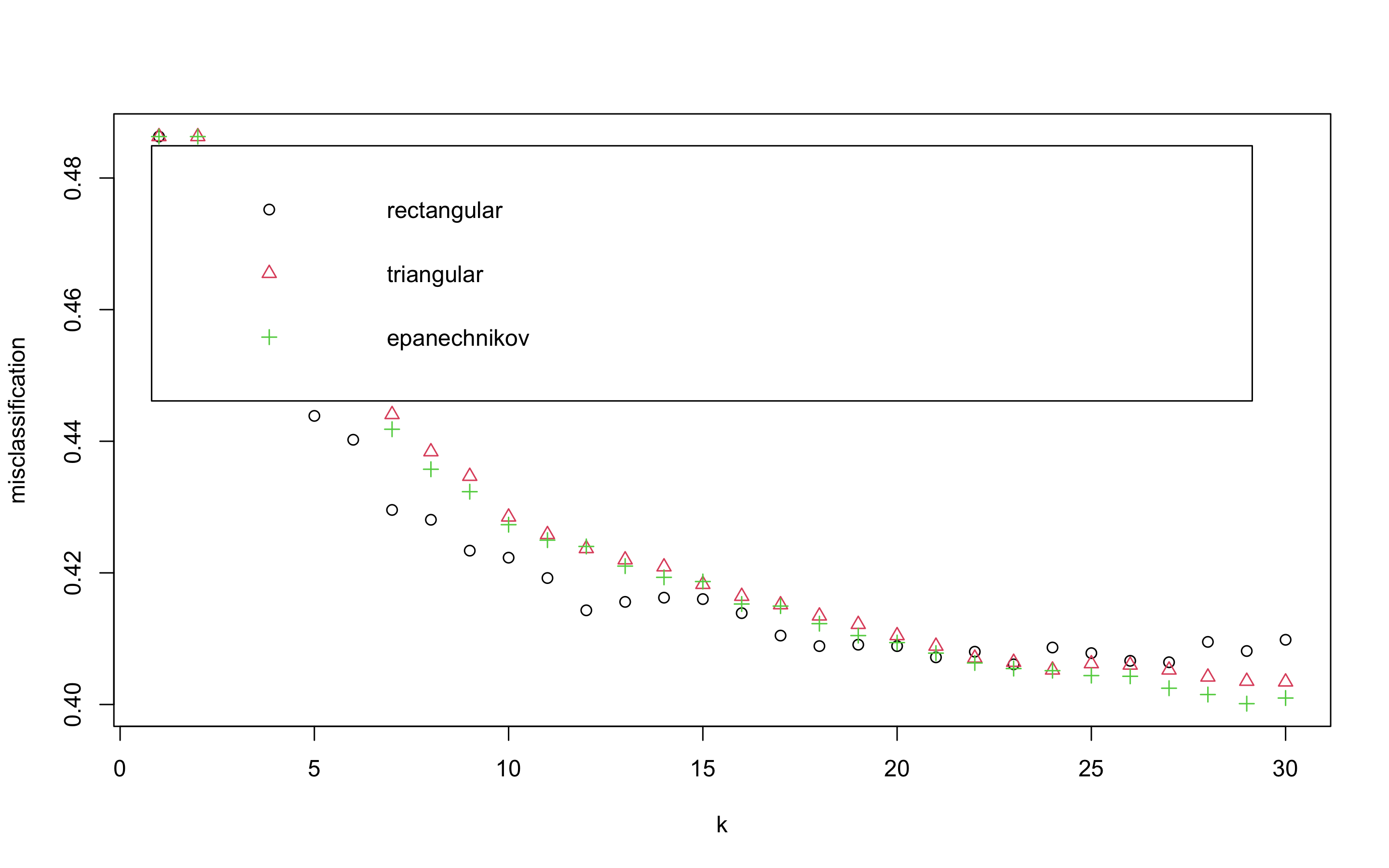
위의 plot은 k값을 x축, 각 커널에 의해 잘못 분류된 관찰값의 비율을 y축에 표시하고 있다. 얼핏보았을 때 k가 29일 때 epanechnikov커널을 사용했을 때 가장 오류가 낮은 것으로 보인다.
- 더 정확히 살펴보자.
> kknn.train

Call:
train.kknn(formula = class ~ ., data = scaled_train_knn, kmax = 30,     distance = 2, kernel = c("rectangular", "triangular", "epanechnikov"))

Type of response variable: nominal
Minimal misclassification: 0.400128
Best kernel: epanechnikov
Best k: 29- 이제 predict함수를 사용해 예측해보자.
> kknn.pred <- predict(kknn.train, newdata = scaled_test_knn)
> confusionMatrix(kknn.pred, scaled_test_knn$class)
Confusion Matrix and Statistics

          Reference
Prediction   A   B   C   D
         A 789 346 146  33
         B 178 441 227 109
         C  23 168 511 232
         D  14  49 120 630

Overall Statistics

               Accuracy : 0.5904
                 95% CI : (0.575, 0.6057)
    No Information Rate : 0.25
    P-Value [Acc > NIR] : < 2.2e-16

                  Kappa : 0.4539

 Mcnemar's Test P-Value : < 2.2e-16

Statistics by Class:

                     Class: A Class: B Class: C Class: D
Sensitivity            0.7859   0.4392   0.5090   0.6275
Specificity            0.8257   0.8293   0.8596   0.9392
Pos Pred Value         0.6005   0.4618   0.5471   0.7749
Neg Pred Value         0.9204   0.8161   0.8400   0.8832
Prevalence             0.2500   0.2500   0.2500   0.2500
Detection Rate         0.1965   0.1098   0.1272   0.1569
Detection Prevalence   0.3272   0.2378   0.2326   0.2024
Balanced Accuracy      0.8058   0.6343   0.6843   0.7834
커널X : (정확도 58.6%, 카파통계량 0.4489), 커널O : (정확도 59%, 카파통계량 0.4539)
커널을 사용했을 때가 커널을 사용하지 않았을 때보다 아주 약간 더 나은 성능을 보이고 있다.
SVM
- SVM분석을 해보자.
- SVM은 scale된 데이터를 사용해야 한다.
- e1071패키지의 tune.svm()함수를 이용해 튜닝 파라미터 및 커널함수를 선택하자.
> library(class)
> library(kknn)
> library(e1071)
> library(caret)
> library(MASS)
> library(kernlab)
> library(corrplot)
> linear.tune <- tune.svm(class ~., data = scaled_train,
+                         kernel = 'linear',
+                         cost = c(0.001, 0.01, 0.1, 0.5, 1, 2, 5, 10))
> summary(linear.tune)

Parameter tuning of ‘svm’:

- sampling method: 10-fold cross validation

- best parameters:
 cost
  0.1

- best performance: 0.4456618

- Detailed performance results:
   cost     error dispersion
1 1e-03 0.4645370 0.01667856
2 1e-02 0.4470478 0.01569832
3 1e-01 0.4456618 0.01619672
4 5e-01 0.4463020 0.01493139
5 1e+00 0.4460888 0.01475279
6 2e+00 0.4466221 0.01448448
7 5e+00 0.4466219 0.01446311
8 1e+01 0.4463021 0.01458349
최적의 cost함수는 0.1로 나왔다.
- predict()함수로 test데이터 예측을 실행해보자.
> best.linear <- linear.tune$best.model
> tune.test <- predict(best.linear, newdata = scaled_test)
> confusionMatrix(tune.test, scaled_test$class)
Confusion Matrix and Statistics

          Reference
Prediction   A   B   C   D
         A 733 301 141  44
         B 252 405 233 118
         C  13 226 410 168
         D   6  72 220 674

Overall Statistics

               Accuracy : 0.5533
                 95% CI : (0.5378, 0.5687)
    No Information Rate : 0.25
    P-Value [Acc > NIR] : < 2.2e-16

                  Kappa : 0.4044

 Mcnemar's Test P-Value : < 2.2e-16

Statistics by Class:

                     Class: A Class: B Class: C Class: D
Sensitivity            0.7301   0.4034   0.4084   0.6713
Specificity            0.8386   0.7998   0.8649   0.9011
Pos Pred Value         0.6013   0.4018   0.5018   0.6934
Neg Pred Value         0.9031   0.8009   0.8143   0.8916
Prevalence             0.2500   0.2500   0.2500   0.2500
Detection Rate         0.1825   0.1008   0.1021   0.1678
Detection Prevalence   0.3035   0.2510   0.2034   0.2420
Balanced Accuracy      0.7844   0.6016   0.6366   0.7862
정확도는 약 55.3%, 카파통계량은 0.4044가 나왔다. KNN분류기 보다 낮은 성능이다.
- polynomial커널함수를 사용해 degree와 커널계수를 조정해보자. degree는 3, 4, 5의 값을 주고 coef0은 0.1부터 4까지의 숫자를 준다.
> set.seed(123)
> poly.tune <- tune.svm(class ~., data = scaled_train,
+                       kernel = 'polynomial', degree = c(3, 4, 5),
+                       coef0 = c(0.1, 0.5, 1, 2, 3, 4))
> summary(poly.tune)

Parameter tuning of ‘svm’:

- sampling method: 10-fold cross validation

- best parameters:
 degree coef0
      3     3

- best performance: 0.3559744

- Detailed performance results:
   degree coef0     error dispersion
1       3   0.1 0.3757039 0.02016595
2       4   0.1 0.3829551 0.01954127
3       5   0.1 0.3956462 0.01639961
4       3   0.5 0.3657837 0.02027498
5       4   0.5 0.3621583 0.02020181
6       5   0.5 0.3646096 0.01985574
7       3   1.0 0.3610916 0.01877135
8       4   1.0 0.3595992 0.01953197
9       5   1.0 0.3683441 0.01915916
10      3   2.0 0.3568267 0.01675985
11      4   2.0 0.3584260 0.01808252
12      5   2.0 0.3664251 0.01715993
13      3   3.0 0.3559744 0.01528650
14      4   3.0 0.3589597 0.01817861
15      5   3.0 0.3664249 0.01730917
16      3   4.0 0.3562944 0.01675393
17      4   4.0 0.3598136 0.01573694
18      5   4.0 0.3669589 0.01575001
최적의 degree는 3이고, coef0은 3이다.
- predict()함수로 test데이터를 사용해 예측을 해보자.
> best.poly <- poly.tune$best.model
> poly.test <- predict(best.poly, newdata = scaled_test)
> confusionMatrix(poly.test, scaled_test$class)
Confusion Matrix and Statistics

          Reference
Prediction   A   B   C   D
         A 823 311 139  43
         B 164 515 202  92
         C   9 145 557 199
         D   8  33 106 670

Overall Statistics

               Accuracy : 0.6387
                 95% CI : (0.6236, 0.6536)
    No Information Rate : 0.25
    P-Value [Acc > NIR] : < 2.2e-16

                  Kappa : 0.5183

 Mcnemar's Test P-Value : < 2.2e-16

Statistics by Class:

                     Class: A Class: B Class: C Class: D
Sensitivity            0.8197   0.5129   0.5548   0.6673
Specificity            0.8363   0.8479   0.8828   0.9512
Pos Pred Value         0.6254   0.5293   0.6121   0.8201
Neg Pred Value         0.9330   0.8393   0.8561   0.8956
Prevalence             0.2500   0.2500   0.2500   0.2500
Detection Rate         0.2049   0.1282   0.1387   0.1668
Detection Prevalence   0.3277   0.2423   0.2266   0.2034
Balanced Accuracy      0.8280   0.6804   0.7188   0.8093
정확도는 약 63.87%이고, 카파통계량은 0.5183이다. 선형 svm모델(정확도 55.3%, 카파통계량 0.4044)보다 훨씬 좋은 성능을 보인다.
- 다음으로 커널 함수로 시그모이드를 설정해보자. 매개변수인 gamma와 coef0이 최적의 값이 되도록 계산해보자.
> set.seed(123)
> sigmoid.tune <- tune.svm(class ~., data = scaled_train,
+                          kernel = 'sigmoid',
+                          gamma = c(0.1, 0.5, 1, 2, 3, 4),
+                          coef0 = c(0.1, 0.5, 1, 2, 3, 4))
> summary(sigmoid.tune)

Parameter tuning of ‘svm’:

- sampling method: 10-fold cross validation

- best parameters:
 gamma coef0
   0.1     4

- best performance: 0.5549702

- Detailed performance results:
   gamma coef0     error  dispersion
1    0.1   0.1 0.6098942 0.017237266
2    0.5   0.1 0.6647129 0.019556511
3    1.0   0.1 0.6778299 0.013018919
4    2.0   0.1 0.6796458 0.013721557
5    3.0   0.1 0.6816705 0.008677423
6    4.0   0.1 0.6800726 0.014748441
7    0.1   0.5 0.6410379 0.016690596
8    0.5   0.5 0.6865779 0.019343938
9    1.0   0.5 0.6830530 0.013403084
10   2.0   0.5 0.6786878 0.018862369
11   3.0   0.5 0.6784731 0.016285652
12   4.0   0.5 0.6816695 0.011816541
13   0.1   1.0 0.6450930 0.017299432
14   0.5   1.0 0.7033180 0.020566970
15   1.0   1.0 0.7010799 0.012793388
16   2.0   1.0 0.6857219 0.010920674
17   3.0   1.0 0.6810307 0.013951721
18   4.0   1.0 0.6827354 0.012767381
19   0.1   2.0 0.6403987 0.018140656
20   0.5   2.0 0.7070483 0.014031467
21   1.0   2.0 0.7103602 0.024367990
22   2.0   2.0 0.6890285 0.014172960
23   3.0   2.0 0.6838045 0.015632352
24   4.0   2.0 0.6862564 0.012334060
25   0.1   3.0 0.6132047 0.016577372
26   0.5   3.0 0.7262468 0.013513776
27   1.0   3.0 0.7068387 0.016881267
28   2.0   3.0 0.6974507 0.014741367
29   3.0   3.0 0.6877478 0.012779387
30   4.0   3.0 0.6875358 0.015403522
31   0.1   4.0 0.5549702 0.024714337
32   0.5   4.0 0.7200590 0.022518266
33   1.0   4.0 0.7127002 0.018309779
34   2.0   4.0 0.7092896 0.010917369
35   3.0   4.0 0.6956382 0.013894373
36   4.0   4.0 0.6910530 0.013037909
_최적의 gamma 값으로 0.1이 선택되었고, coef0 값으로는 4가 선택되었다.
- 이제 예측을 해보자.
> best.sigmoid <- sigmoid.tune$best.model
> sigmoid.test <- predict(best.sigmoid, newdata = scaled_test)
> confusionMatrix(sigmoid.test, scaled_test$class)
Confusion Matrix and Statistics

          Reference
Prediction   A   B   C   D
         A 943 708 457 154
         B   0   0   0   0
         C  21  68 121  59
         D  40 228 426 791

Overall Statistics

               Accuracy : 0.4619
                 95% CI : (0.4464, 0.4775)
    No Information Rate : 0.25
    P-Value [Acc > NIR] : < 2.2e-16

                  Kappa : 0.2825

 Mcnemar's Test P-Value : < 2.2e-16

Statistics by Class:

                     Class: A Class: B Class: C Class: D
Sensitivity            0.9392     0.00  0.12052   0.7878
Specificity            0.5621     1.00  0.95086   0.7696
Pos Pred Value         0.4169      NaN  0.44981   0.5327
Neg Pred Value         0.9652     0.75  0.76434   0.9158
Prevalence             0.2500     0.25  0.25000   0.2500
Detection Rate         0.2348     0.00  0.03013   0.1970
Detection Prevalence   0.5632     0.00  0.06698   0.3698
Balanced Accuracy      0.7507     0.50  0.53569   0.7787
정확도는 약 46.19%, 카파통계량은 약 0.2825로 가장 좋지 않은 성능을 보인다.
현재까지는 polynomial커널함수를 사용한 SVM모델이 정확도 63.87%, 카파통계량 0.5183로 가장 좋은 성능을 보이고 있다.
랜덤포레스트
- 다음으로 랜덤포레스트 모델을 만들어 보자.
> library(rpart)
> library(partykit)
> library(MASS)
> library(genridge)
> library(randomForest)
> library(xgboost)
> library(caret)
> library(Boruta)
> rfmodel <- randomForest(class ~., data = train)
> rfmodel

Call:
 randomForest(formula = class ~ ., data = train)
               Type of random forest: classification
                     Number of trees: 500
No. of variables tried at each split: 3

        OOB estimate of  error rate: 30.89%
Confusion matrix:
     A    B    C    D class.error
A 1948  326   52   18   0.1689420
B  613 1286  308  136   0.4511310
C  295  457 1401  192   0.4025586
D   50  166  284 1845   0.2132196
수행 결과 OOB(out of bag)오차율은 30.89%가 나왔다.
- 개선을 위해 최적의 트리수를 보자.
> plot(rfmodel)
> which.min(rfmodel$err.rate[, 1])
[1] 401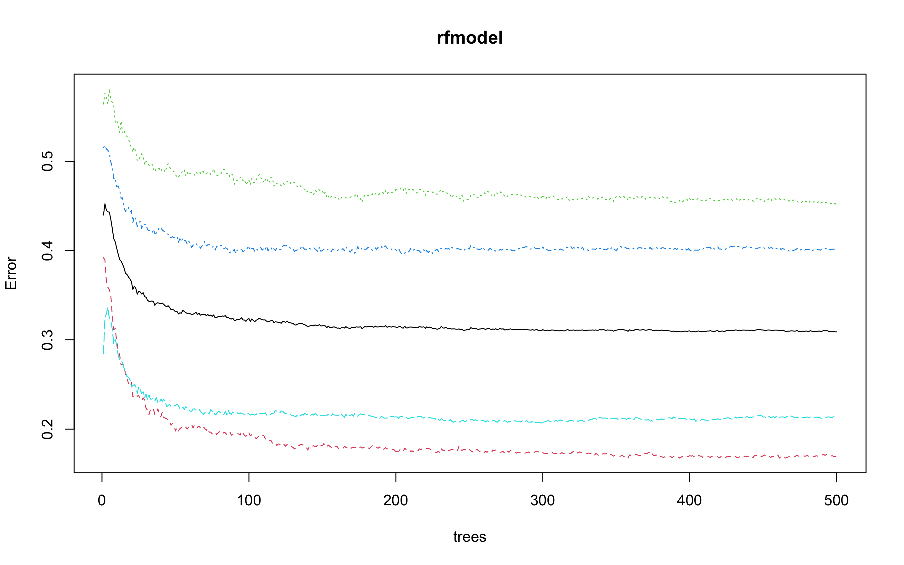
모형 정확도를 최적화하기에 필요한 트리수가 401개면 된다는 결과를 얻었다.
> set.seed(123)
> rfmodel2 <- randomForest(class ~., data = train, ntree = 401)
> rfmodel2

Call:
 randomForest(formula = class ~ ., data = train, ntree = 401)
               Type of random forest: classification
                     Number of trees: 401
No. of variables tried at each split: 3

        OOB estimate of  error rate: 30.88%
Confusion matrix:
     A    B    C    D class.error
A 1946  326   54   18   0.1697952
B  614 1277  318  134   0.4549723
C  289  452 1407  197   0.4000000
D   53  160  281 1851   0.2106610
OOB 오차율이 30.89%에서 30.88%로 미미한 차이를 보인다.
- test데이터로 어떤 결과가 나오는지 보자.
> rftest <- predict(rfmodel2, newdata = test, type = 'response')
> confusionMatrix(rftest, test$class)
Confusion Matrix and Statistics

          Reference
Prediction   A   B   C   D
         A 851 262 104  24
         B 127 546 204  59
         C  18 139 586 111
         D   8  57 110 810

Overall Statistics

               Accuracy : 0.6955
                 95% CI : (0.681, 0.7097)
    No Information Rate : 0.25
    P-Value [Acc > NIR] : < 2.2e-16

                  Kappa : 0.594

 Mcnemar's Test P-Value : < 2.2e-16

Statistics by Class:

                     Class: A Class: B Class: C Class: D
Sensitivity            0.8476   0.5438   0.5837   0.8068
Specificity            0.8705   0.8705   0.9110   0.9419
Pos Pred Value         0.6857   0.5833   0.6862   0.8223
Neg Pred Value         0.9449   0.8513   0.8678   0.9360
Prevalence             0.2500   0.2500   0.2500   0.2500
Detection Rate         0.2119   0.1360   0.1459   0.2017
Detection Prevalence   0.3090   0.2331   0.2126   0.2453
Balanced Accuracy      0.8591   0.7072   0.7473   0.8743
정확도 69.55%, 카파통계량 0.594로 polynomial커널함수를 사용한 SVM모델(정확도 63.87%, 카파통계량 0.5183)보다 좋은 성능을 보인다.
익스트림 그레디언트 부스트
- 다음으로 익스트림 그레디언트 부스트 모델을 만들어 보자.
- 먼저 train데이터와 test데이터를 더미 변수로 바꿔주자.
> dummies <- dummyVars(class ~., data = train)
> dummies
Dummy Variable Object

Formula: class ~ .
10 variables, 2 factors
Variables and levels will be separated by '.'
A less than full rank encoding is used
> train_dummies <- as.data.frame(predict(dummies, newdata = train))
Warning message:
In model.frame.default(Terms, newdata, na.action = na.action, xlev = object$lvls) :
  variable 'class' is not a factor
> str(train_dummies)
'data.frame':	9377 obs. of  10 variables:
 $ age                    : num  25 31 32 42 57 27 22 24 25 26 ...
 $ height_cm              : num  165 180 174 164 162 ...
 $ weight_kg              : num  55.8 78 71.1 63.7 58.2 53.9 67.9 84.4 66.6 71.5 ...
 $ body.fat_.             : num  15.7 20.1 18.4 32.2 20.9 35.5 18 20.4 30.2 18 ...
 $ diastolic              : num  77 92 76 72 69 69 71 80 82 64 ...
 $ systolic               : num  126 152 147 135 106 116 120 120 120 135 ...
 $ sit.and.bend.forward_cm: num  16.3 12 15.2 0.8 20.7 13.1 19.2 7.2 22.9 17.8 ...
 $ sit.ups.counts         : num  53 49 53 18 30 28 55 54 39 50 ...
 $ gender.F               : num  0 0 0 1 1 1 0 0 1 0 ...
 $ gender.M               : num  1 1 1 0 0 0 1 1 0 1 ...
> train_dummies$class <- train$class

> dummies2 <- dummyVars(class ~., data = test)
> dummies2
Dummy Variable Object

Formula: class ~ .
10 variables, 2 factors
Variables and levels will be separated by '.'
A less than full rank encoding is used
> test_dummies <- as.data.frame(predict(dummies2, newdata = test))
Warning message:
In model.frame.default(Terms, newdata, na.action = na.action, xlev = object$lvls) :
  variable 'class' is not a factor
> str(test_dummies)
'data.frame':	4016 obs. of  10 variables:
 $ age                    : num  27 28 36 33 54 28 42 45 38 23 ...
 $ height_cm              : num  172 174 165 175 167 ...
 $ weight_kg              : num  75.2 67.7 55.4 77.2 67.5 ...
 $ body.fat_.             : num  21.3 17.1 22 28 27.6 14.4 19.3 30.9 23.2 29.6 ...
 $ diastolic              : num  80 70 64 84 85 81 63 93 70 91 ...
 $ systolic               : num  130 127 119 137 141 141 110 144 111 126 ...
 $ sit.and.bend.forward_cm: num  18.4 20.7 21 12.3 18.6 12.1 16 19 19.7 20.7 ...
 $ sit.ups.counts         : num  60 45 27 42 34 55 50 30 50 32 ...
 $ gender.F               : num  0 0 1 0 0 0 0 1 0 1 ...
 $ gender.M               : num  1 1 0 1 1 1 1 0 1 0 ...
> test_dummies$class <- test$class- 부스트 기법을 사용하기 위해서는 여러 인자값들을 세부 조정해야 한다.
- 그리드를 만들어 보자.
- 각 인자값들은 다음과 같다.
| 인자 | Description |
|---|---|
| nrounds | 최대 반복 횟수(최종 모형에서의 트리 수) |
| colsample_bytree | 트리를 생성할 때 표본 추출할 피처 수(비율로 표시됨), 기본값은 1 |
| min_child_weight | 부스트되는 트리에서 최소 가중값, 기본값은 1 |
| eta | 학습 속도, 해법에 관한 각 트리의 기여도를 의미, 기본값은 0.3 |
| gamma | 트리에서 다른 leaf 분할을 하기 위해 필요한 최소 손실 감소 |
| subsample | 데이터 관찰값의 비율, 기본값은 1 |
| max_depth | 개별 트리의 최대 깊이 |
> grid <- expand.grid(nrounds = c(350, 500),
+                     colsample_bytree = 1,
+                     min_child_weight = 1,
+                     eta = c(0.01, 0.1, 0.3),
+                     gamma = c(0.5, 0.25),
+                     subsample = 0.5,
+                     max_depth = c(2, 3)
+ )- trainControl인자를 조정한다. 여기서는 5-fold 교차검증을 사용할 것이다.
> cntrl <- trainControl(method = 'cv',
+                       number = 5,
+                       verboseIter = TRUE,
+                       returnData = FALSE,
+ returnResamp = 'final')- train()을 사용해 train데이터를 학습시킨다.
> train.xgb <- train(x = train_dummies[, 1:10],
+                    y = train_dummies[, 11],
+                    trControl = cntrl,
+                    tuneGrid = grid,
+                    method = 'xgbTree')
+ Fold1: eta=0.01, max_depth=2, gamma=0.25, colsample_bytree=1, min_child_weight=1, subsample=0.5, nrounds=500
[16:31:08] WARNING: amalgamation/../src/c_api/c_api.cc:718: `ntree_limit` is deprecated, use `iteration_range` instead.
- Fold1: eta=0.01, max_depth=2, gamma=0.25, colsample_bytree=1, min_child_weight=1, subsample=0.5, nrounds=500
.
.
.
- Fold5: eta=0.30, max_depth=3, gamma=0.50, colsample_bytree=1, min_child_weight=1, subsample=0.5, nrounds=500
Aggregating results
Selecting tuning parameters
Fitting nrounds = 350, max_depth = 3, eta = 0.1, gamma = 0.25, colsample_bytree = 1, min_child_weight = 1, subsample = 0.5 on full training set
상당히 긴 출력이 나오기 때문에 중간의 출력은 생략했다.
최적 인자들의 조합으로 nrounds = 350, max_depth = 3, eta = 0.1, gamma = 0.25, colsample_bytree = 1, min_child_weight = 1, subsample = 0.5이 선택되었다.
- xgb.train()에서 사용할 인자 목록을 생성하고, 데이터 프레임을 입력피처의 행렬과 숫자 레이블의 목록으로 변환한다. 그런 다음, 피처와 식별값을 xgb.DMatrix에서 사용할 입력값으로 변환한다.
> param <- list(booster = "gbtree",
+      objective = "multi:softprob",
+      num_class = 4,
+      eval_metric = 'error',
+      eta = 0.1,
+      max_depth = 3,
+      subsample = 0.5,
+      colsample_bytree = 1,
+      gamma = 0.25)
> x <- as.matrix(train_dummies[, 1:10])
> train.mat <- xgb.DMatrix(data = x, label = as.numeric(train_dummies$class) - 1)- 이제 모형을 만들어 보자.
> set.seed(321)
> xgb.fit <- xgb.train(params = param, data = train.mat, nrounds = 350)- test데이터에 관한 결과를 보기 전에 변수 중요도를 그려 검토해보자.
- 항목은 gain, cover, frequency 이렇게 세가지를 검사할 수 있다. gain은 피처가 트리에 미치는 정확도의 향상 정도를 나타내는 값, cover는 이 피처와 연관된 전체 관찰값의 상대 수치, frequency는 모든 트리에 관해 피처가 나타난 횟수를 백분율로 나타낸 값이다.
impMatrix <- xgb.importance(feature_names = dimnames(x)[[2]], model = xgb.fit)
impMatrix
xgb.plot.importance(impMatrix, main = 'Gain by Feature')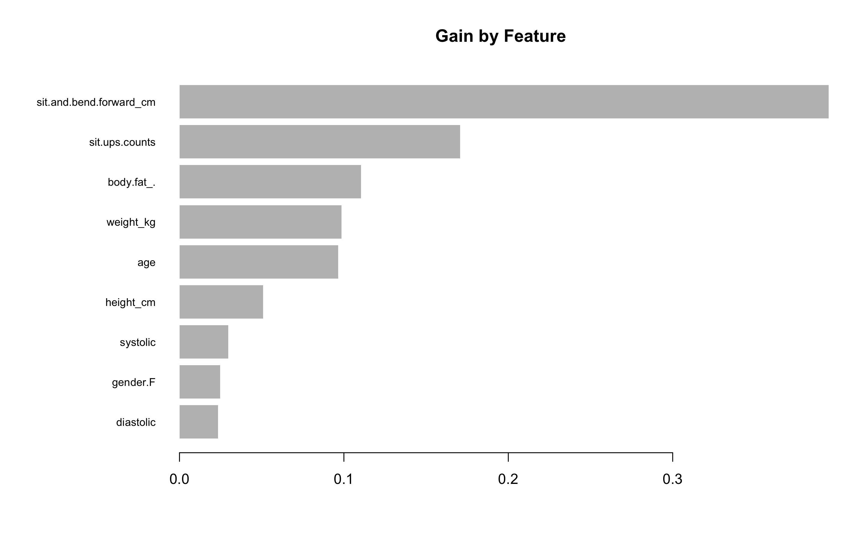
- 다음으로 test데이터에 관한 수행 결과를 보자.
> library(InformationValue)
> pred <- predict(xgb.fit, x)
> optimalCutoff(y, pred)
[1] 0.4399996
> testMat <- as.matrix(test_dummies[, 1:10])
> xgb.test <- predict(xgb.fit, testMat)
> y.test <- as.numeric(test_dummies$class) - 1
> confusionMatrix(y.test, xgb.test, threshold = 0.4399)
Error in table(predicted_dir, actual_dir) :
  all arguments must have the same length
> 1 - misClassError(y.test, xgb.test, threshold = 0.4399)
[1] -2
> plotROC(y.test, xgb.test)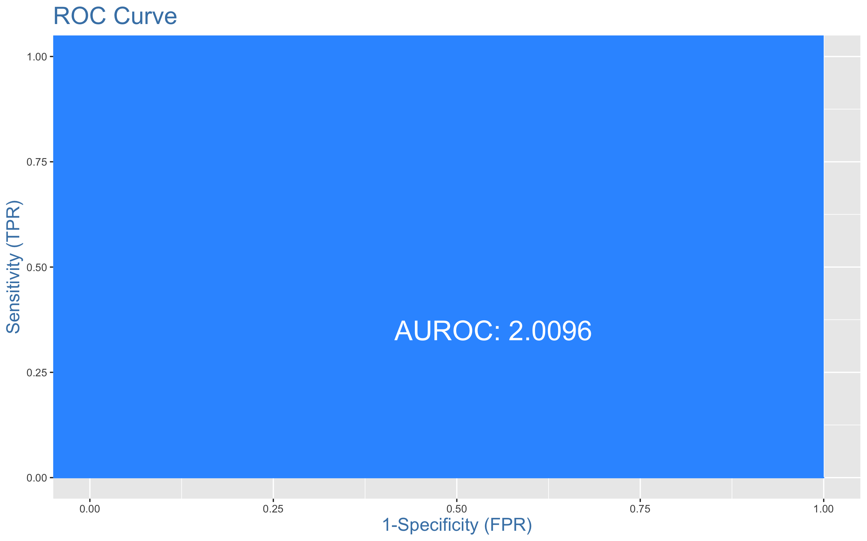
AUC의 최댓값은 1로 알고 있었다... 하지만 2.0096이 나왔지... 무엇이 문제일까??
앙상블 분석
- 앙상블 분석을 해보자
> library(caret)
> library(MASS)
> library(caretEnsemble)
> library(caTools)
> library(mlr)
> library(ggplot2)
> library(HDclassif)
> library(reshape2)
> library(corrplot)
> library(gbm)
> library(mboost)
> control <- trainControl(method = 'cv', number = 5,
+                         savePredictions = 'final',
+                         classProbs = TRUE,
+                         summaryFunction = defaultSummary)
> set.seed(1234)
> models <- caretList(class ~., data = train,
+                     trControl = control,
+                     metric = 'ROC',
+                     methodList = c('rpart', 'earth', 'knn'))
There were 28 warnings (use warnings() to see them)
> models
$rpart
CART

9377 samples
   9 predictor
   4 classes: 'A', 'B', 'C', 'D'

No pre-processing
Resampling: Cross-Validated (5 fold)
Summary of sample sizes: 7503, 7501, 7501, 7502, 7501
Resampling results across tuning parameters:

  cp          Accuracy   Kappa
  0.02531286  0.4917378  0.3223165
  0.06214448  0.4499429  0.2665902
  0.20221843  0.4134534  0.2179368

Accuracy was used to select the optimal model using the largest value.
The final value used for the model was cp = 0.02531286.

$earth
Multivariate Adaptive Regression Spline

9377 samples
   9 predictor
   4 classes: 'A', 'B', 'C', 'D'

No pre-processing
Resampling: Cross-Validated (5 fold)
Summary of sample sizes: 7503, 7501, 7501, 7502, 7501
Resampling results across tuning parameters:

  nprune  Accuracy   Kappa
   2      0.4363864  0.2484982
   8      0.5503914  0.4005246
  14      0.5748124  0.4330834

Tuning parameter 'degree' was held constant at a value of 1
Accuracy was used to select the optimal model using the largest value.
The final values used for the model were nprune = 14 and degree = 1.

$knn
k-Nearest Neighbors

9377 samples
   9 predictor
   4 classes: 'A', 'B', 'C', 'D'

No pre-processing
Resampling: Cross-Validated (5 fold)
Summary of sample sizes: 7503, 7501, 7501, 7502, 7501
Resampling results across tuning parameters:

  k  Accuracy   Kappa
  5  0.5325800  0.3767785
  7  0.5415352  0.3887178
  9  0.5506006  0.4008056

Accuracy was used to select the optimal model using the largest value.
The final value used for the model was k = 9.

attr(,"class")
[1] "caretList"- 모형끼리 상호연관성이 어떤지 살펴보자.
> modelCor(resamples(models))
           rpart      earth        knn
rpart  1.0000000  0.8561974 -0.7627144
earth  0.8561974  1.0000000 -0.6274591
knn   -0.7627144 -0.6274591  1.0000000
효과적인 앙상블을 위해서는 상호연관성이 높지 않은 것이 좋다. rpart와 earth, knn과 rpart의 상호 연관성이 다소 높아 보인다.
- 다른 앙상블 조합을 시도해보자.
> set.seed(1234)
> models <- caretList(class ~., data = train,
+                     trControl = control,
+                     metric = 'ROC',
+                     methodList = c('treebag', 'earth', 'knn'))
There were 28 warnings (use warnings() to see them)
> models
$treebag
Bagged CART

9377 samples
   9 predictor
   4 classes: 'A', 'B', 'C', 'D'

No pre-processing
Resampling: Cross-Validated (5 fold)
Summary of sample sizes: 7503, 7501, 7501, 7502, 7501
Resampling results:

  Accuracy   Kappa
  0.6641765  0.5522371


$earth
Multivariate Adaptive Regression Spline

9377 samples
   9 predictor
   4 classes: 'A', 'B', 'C', 'D'

No pre-processing
Resampling: Cross-Validated (5 fold)
Summary of sample sizes: 7503, 7501, 7501, 7502, 7501
Resampling results across tuning parameters:

  nprune  Accuracy   Kappa
   2      0.4363864  0.2484982
   8      0.5503914  0.4005246
  14      0.5748124  0.4330834

Tuning parameter 'degree' was held constant at a value of 1
Accuracy was used to select the optimal model using the largest value.
The final values used for the model were nprune = 14 and degree = 1.

$knn
k-Nearest Neighbors

9377 samples
   9 predictor
   4 classes: 'A', 'B', 'C', 'D'

No pre-processing
Resampling: Cross-Validated (5 fold)
Summary of sample sizes: 7503, 7501, 7501, 7502, 7501
Resampling results across tuning parameters:

  k  Accuracy   Kappa
  5  0.5303412  0.3737935
  7  0.5402554  0.3870114
  9  0.5516674  0.4022275

Accuracy was used to select the optimal model using the largest value.
The final value used for the model was k = 9.

attr(,"class")
[1] "caretList"
> modelCor(resamples(models))
          treebag      earth        knn
treebag 1.0000000  0.0385026  0.1967112
earth   0.0385026  1.0000000 -0.5078148
knn     0.1967112 -0.5078148  1.0000000
상호연관성이 낮아보인다.
> model_preds <- lapply(models, predict, newdata = test, type = 'prob')
> model_preds <- lapply(model_preds, function(x) x[, 'A'])
> model_preds <- data.frame(model_preds)
> stack <- caretStack(models, method = 'glm', metric = 'ROC',
+                     trControl = trainControl(
+                       method = 'boot', number = 5,
+                       savePredictions = 'final',
+                       classProbs = TRUE,
+                       summaryFunction = defaultSummary
+                     ))
Error in check_caretList_model_types(list_of_models) :
  Not yet implemented for multiclass problems
caretStack은 multiclass모델에 관해서는 지원하지 않나보다...이럴수가
Conclusion
다중 분류는 너무 어렵다... 익스트림 그레디언트 부스트와 앙상블 분석에서는 제대로 된 결론도 못 내렸다.
다중 분류를 아예 지원하지 않는 패키지도 많고, 정확한 AUC도 구하기 어려웠다...
그렇다면 다중분류를 이중분류로 사용해서 분석하면 어떨까?
A, B, C, D의 분류가 있으면 A를 Good으로 바꾸고 B, C, D를 Bad로 바꾸는 것이다. 혹은 A, B를 Good으로 C, D를 Bad로 재할당해서 다시 데이터 분석을 해봐야겠다.
_'Body Performance Data'를 이용한 분류분석_ver2로 다시 찾아오겠다...ver2_click!
사용한 패키지
pastecs, psych, PerformanceAnalytics, caret, GGally, reshape2, ggplot2, gridExtra, gapminder, dplyr, class, kknn, e1071, MASS, kernlab, corrplot, rpart, partykit, genridge, randomForest, xgboost, Boruta, InformationValue,
caretEnsemble, caTools, mlr, HDclassif, gbm, mboost