Air pollution Forecasting LSTM

필수 모듈을 불러온다 .

import pandas as pd
import numpy as np
import matplotlib.pyplot as plt
import tensorflow as tf
import seaborn as sns
from sklearn.metrics import mean_absolute_error , mean_squared_error
from sklearn.preprocessing import MinMaxScaler
from sklearn.preprocessing import LabelEncoder
from tensorflow.keras.layers import LSTM, Dense, Dropout, BatchNormalization
from tensorflow.keras.models import Sequential

데이터를 불러온다.

df = pd.read_csv('LSTM-Multivariate_pollution.csv')
df

>>>	date	pollution	dew	temp	press	wnd_dir	wnd_spd	snow	rain
0	2010-01-02 00:00:00	129.0	-16	-4.0	1020.0	SE	1.79	0	0
1	2010-01-02 01:00:00	148.0	-15	-4.0	1020.0	SE	2.68	0	0
2	2010-01-02 02:00:00	159.0	-11	-5.0	1021.0	SE	3.57	0	0
3	2010-01-02 03:00:00	181.0	-7	-5.0	1022.0	SE	5.36	1	0
4	2010-01-02 04:00:00	138.0	-7	-5.0	1022.0	SE	6.25	2	0
...	...	...	...	...	...	...	...	...	...
43795	2014-12-31 19:00:00	8.0	-23	-2.0	1034.0	NW	231.97	0	0
43796	2014-12-31 20:00:00	10.0	-22	-3.0	1034.0	NW	237.78	0	0
43797	2014-12-31 21:00:00	10.0	-22	-3.0	1034.0	NW	242.70	0	0
43798	2014-12-31 22:00:00	8.0	-22	-4.0	1034.0	NW	246.72	0	0
43799	2014-12-31 23:00:00	12.0	-21	-3.0	1034.0	NW	249.85	0	0
43800 rows × 9 columns

문자열 데이터를 확인하고 숫자로 변환해준다.

df["wnd_dir"].unique()

>>> array(['SE', 'cv', 'NW', 'NE'], dtype=object)

def func(s):
    if s == "SE":
        return 1
    elif s == "NE":
        return 2
    elif s == "NW":
        return 3
    else:
        return 4

df["wind_dir"] = df["wnd_dir"].apply(func)

del df["wnd_dir"]

각 컬럼들을 시각적으로 변환하여 본다.

values = df.values

# specify columns to plot
groups = [1, 2, 3, 5, 6]
i = 1

# plot each column
plt.figure(figsize=(20,14))
for group in groups:
    plt.subplot(len(groups), 1, i)
    plt.plot(values[:, group], c = "forestgreen")
    plt.title(df.columns[group], y=0.75, loc='right', fontsize = 15)
    i += 1
plt.show()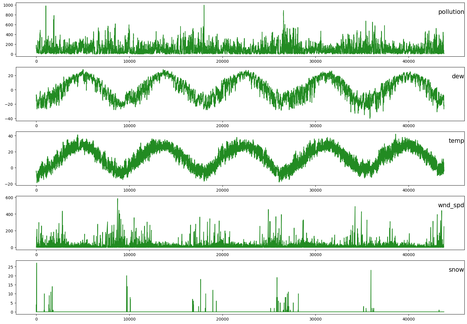

지정된 시간에 걸친 오염 변화를 확인하여 준다.

fig = plt.figure(figsize = (20,7))
plt.plot(df.pollution)
plt.title("Polution variation across the given no of hours", fontsize = 15)
plt.show()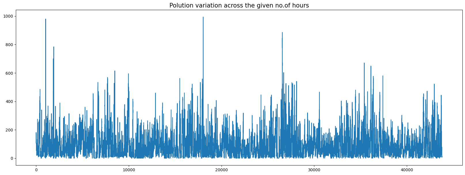

데이터를 정리하고

del df["date"]

데이터프레임의 값을 불러오고 실수형으로 변환한다.
MinMaxScaler를 통해 데이터를 스케일링해준다.
MinMaxScaler는 데이터 값을 0~1사이의 값으로 변환해주며 음수값이 있으면 -1에서 1값으로 변환한다. 데이터의 분포가 정규분포(가우시안 분포)가 아닐경우 적용해 볼 수 있다.

dataset = df
values = dataset.values

values = values.astype('float32')

scaler = MinMaxScaler(feature_range=(0, 1))
scaled = scaler.fit_transform(values)

샘플의 입력층을 3차원으로 변환하기 위한 함수를 구성한다.

def series_to_supervised(data, n_in = 1, n_out = 1, dropnan = True):
    n_vars = 1 if type(data) is list else data.shape[1]
    
    df = pd.DataFrame(data)
    cols, names = list(), list()
    
    # input sequence (t-n, ... t-1)
    for i in range(n_in, 0, -1):
        cols.append(df.shift(i))
        names += [('var%d(t-%d)' % (j+1, i)) for j in range(n_vars)]
        
    # forecast sequence (t, t+1, ... t+n)
    for i in range(0, n_out):
        cols.append(df.shift(-i))
        if i == 0:
            names += [('var%d(t)' % (j+1)) for j in range(n_vars)]
        else:
            names += [('var%d(t+%d)' % (j+1, i)) for j in range(n_vars)]
            
    # put it all together
    agg = pd.concat(cols, axis=1)
    agg.columns = names
    # drop rows with NaN values
    if dropnan:
        agg.dropna(inplace=True)
        
    return agg

스케일된 데이터프레임을 3차원으로 만드는 함수를 통해 재구성한다.

reframed = series_to_supervised(scaled, 1, 1)
print(reframed.shape)

>>>(43799, 16)

print(reframed.head())

>>> var1(t-1)  var2(t-1)  var3(t-1)  var4(t-1)  var5(t-1)  var6(t-1)  \
1   0.129779   0.352941   0.245902   0.527273   0.002290   0.000000   
2   0.148893   0.367647   0.245902   0.527273   0.003811   0.000000   
3   0.159960   0.426471   0.229508   0.545454   0.005332   0.000000   
4   0.182093   0.485294   0.229508   0.563637   0.008391   0.037037   
5   0.138833   0.485294   0.229508   0.563637   0.009912   0.074074   

   var7(t-1)  var8(t-1)   var1(t)   var2(t)   var3(t)   var4(t)   var5(t)  \
1        0.0        0.0  0.148893  0.367647  0.245902  0.527273  0.003811   
2        0.0        0.0  0.159960  0.426471  0.229508  0.545454  0.005332   
3        0.0        0.0  0.182093  0.485294  0.229508  0.563637  0.008391   
4        0.0        0.0  0.138833  0.485294  0.229508  0.563637  0.009912   
5        0.0        0.0  0.109658  0.485294  0.213115  0.563637  0.011433   

    var6(t)  var7(t)  var8(t)  
1  0.000000      0.0      0.0  
2  0.000000      0.0      0.0  
3  0.037037      0.0      0.0  
4  0.074074      0.0      0.0  
5  0.111111      0.0      0.0 

reframed.columns

>>>Index(['var1(t-1)', 'var2(t-1)', 'var3(t-1)', 'var4(t-1)', 'var5(t-1)',
       'var6(t-1)', 'var7(t-1)', 'var8(t-1)', 'var1(t)', 'var2(t)', 'var3(t)',
       'var4(t)', 'var5(t)', 'var6(t)', 'var7(t)', 'var8(t)'],
      dtype='object')

인풋할 부분이 아닌 예측할 부분을 제외해 준다.

reframed.drop(reframed.columns[[9,10,11,12,13,14,15]], axis=1, inplace=True)
print(reframed.head())

>>>  var1(t-1)  var2(t-1)  var3(t-1)  var4(t-1)  var5(t-1)  var6(t-1)  \
1   0.129779   0.352941   0.245902   0.527273   0.002290   0.000000   
2   0.148893   0.367647   0.245902   0.527273   0.003811   0.000000   
3   0.159960   0.426471   0.229508   0.545454   0.005332   0.000000   
4   0.182093   0.485294   0.229508   0.563637   0.008391   0.037037   
5   0.138833   0.485294   0.229508   0.563637   0.009912   0.074074   

   var7(t-1)  var8(t-1)   var1(t)  
1        0.0        0.0  0.148893  
2        0.0        0.0  0.159960  
3        0.0        0.0  0.182093  
4        0.0        0.0  0.138833  
5        0.0        0.0  0.109658

트레인하고 테스트할 부분을 나눠준다.
3년만큼의 데이터를 학습하고 나머지 부분을 예측하고 비교하기로 한다.

values = reframed.values

# We train the model on the 1st 3 years and then test on the last year (for now)
n_train_hours = 365 * 24 * 3

train = values[:n_train_hours, :]
test = values[n_train_hours:, :]

# split into input and outputs
train_X, train_y = train[:, :-1], train[:, -1]
test_X, test_y = test[:, :-1], test[:, -1]

# reshape input to be 3D :- (no.of samples, no.of timesteps, no.of features)
train_X = train_X.reshape((train_X.shape[0], 1, train_X.shape[1]))
test_X = test_X.reshape((test_X.shape[0], 1, test_X.shape[1]))
print(train_X.shape, train_y.shape, test_X.shape, test_y.shape)

>>>(26280, 1, 8) (26280,) (17519, 1, 8) (17519,)

train.shape, test.shape, values.shape
>>>((26280, 9), (17519, 9), (43799, 9))

아키텍처 구성: LSTM모델을 어떤 방식으로 쌓을 것인지 정한다.
케라스 모델의 Sequential()을 통해 모델의 설계도를 작성한다.
어떤 식으로 문제를 학습할지에 대한 알고리즘 설계이다.
Sequential 모델은 레이어를 선형으로 연결하여 구성한다.
레이어 인스턴스를 생성자에게 넘겨줌으로써 Sequential 모델을 구성할 수 있다.
여기에 .add( ) 메소드로 레이어를 추가할 수 있다.
에포크를 50번 시행시킨다.

model.add(LSTM( ))

https://www.tensorflow.org/api_docs/python/tf/keras/layers/LSTM

model.add(Dense( ))
: 모든 입력 뉴런과 출력 뉴런을 연결하는 전결합층이다.

https://zereight.tistory.com/227

batch size: total number of training examples present in a single batch
즉, 한 번의 batch마다 주는 데이터의 샘플 사이즈

iteration: the number of passes to complete one epoch
즉, epoch를 나누어서 실행하는 횟수

model = Sequential()
model.add(LSTM(64, input_shape=(train_X.shape[1], train_X.shape[2])))
model.add(Dense(1))
model.compile(loss='mse', optimizer='adam')

# fit network
history = model.fit(train_X, train_y, epochs=50, batch_size=72, validation_split=0.2, verbose=2, shuffle=False)

에포크는 한번을 학습시겠다고 한 것을 실행시키는 것이다.
epoch가 너무 작으면 과소적합, 너무 크면 과대적합의 문제가 있으므로 적절한 epoch 값을 설정해야한다.

※ forward pass: 파라미터를 사용해 입력부터 출력까지 각 계층의 weight를 계산하는 과정
※ backward pass: 반대로 거슬러 올라가면서 다시 한 번 계산 과정을 거쳐 기존의 weight를 수정함
이 두 가지를 수행하면서 weight 값을 찾아가는 것을 backpropagation algorithm이라고 함

Epoch 46/50
292/292 - 0s - loss: 8.1560e-04 - val_loss: 5.6999e-04 - 361ms/epoch - 1ms/step
Epoch 47/50
292/292 - 0s - loss: 8.1514e-04 - val_loss: 5.7015e-04 - 369ms/epoch - 1ms/step
Epoch 48/50
292/292 - 0s - loss: 8.1469e-04 - val_loss: 5.7034e-04 - 417ms/epoch - 1ms/step
Epoch 49/50
292/292 - 0s - loss: 8.1424e-04 - val_loss: 5.7054e-04 - 365ms/epoch - 1ms/step
Epoch 50/50
292/292 - 0s - loss: 8.1381e-04 - val_loss: 5.7072e-04 - 404ms/epoch - 1ms/step

파이플롯을 통해서 트레인과 테스트 데이터를 시각화한다.

plt.figure(figsize=(15,6))
plt.plot(history.history['loss'], label='train', linewidth = 2.5)
plt.plot(history.history['val_loss'], label='test',  linewidth = 2.5)
plt.legend()
plt.show()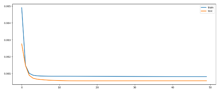

테스트의 쉐잎을 확인한다.

test_X.shape

>>>(17519, 1, 8)

파이썬 매서드 predict()을 통해 예측결과를 반환하고
넘파이 함수 ravel()을 통해 평평하게 배열해준다.

testPredict = model.predict(test_X)
print(testPredict.shape)
testPredict = testPredict.ravel()

print(testPredict.shape)

>>>548/548 [==============================] - 1s 868us/step
>>>(17519, 1)
>>>(17519,)

test.shape
>>>(17519, 9)

print(test), print(test.shape)
>>>[[0.03521127 0.44117647 0.22950819 ... 0.         0.6666666  0.03118712]
 [0.03118712 0.4264706  0.1967213  ... 0.         0.6666666  0.03219316]
 [0.03219316 0.4264706  0.1967213  ... 0.         0.6666666  0.02112676]
 ...
 [0.01006036 0.2647059  0.26229507 ... 0.         0.6666666  0.01006036]
 [0.01006036 0.2647059  0.26229507 ... 0.         0.6666666  0.00804829]
 [0.00804829 0.2647059  0.24590163 ... 0.         0.6666666  0.01207243]]
(17519, 9)
>>>(None, None)

y_test_true = test[:,8]

정확한 오차를 시각화하기 위해 test[:, 8]의 표준편차를 곱하고 이에 평균을 더한다.

poll = np.array(df["pollution"])

meanop = poll.mean()
stdop = poll.std()

y_test_true = y_test_true*stdop + meanop
testPredict = testPredict*stdop + meanop

from matplotlib import pyplot as plt

plt.figure(figsize=(15,6))
plt.xlim([1000,1250])
plt.ylabel("ppm")
plt.xlabel("hrs")
plt.plot(y_test_true, c = "g", alpha = 0.90, linewidth = 2.5)
plt.plot(testPredict, c = "b", alpha = 0.75)
plt.title("Testing(Validation) data")
plt.show()

# testTrue = scaler.inverse_transform([testY]).ravel()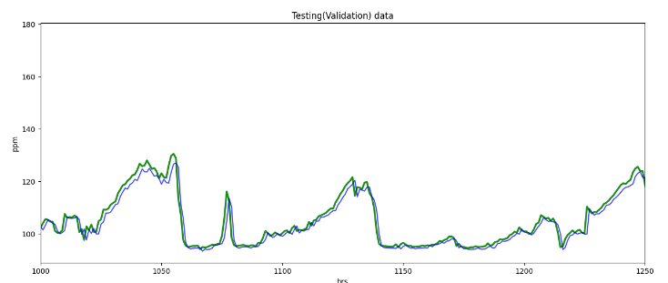

평균 제곱근 오차(RMSE)는 회귀 예측 모델에 대한 두 개의 주요 성과 지표 중 하나로 평균 제곱근 오차는 예측 모델에서 예측한 값과 실제 값 사이의 평균 차이를 측정한다. 예측 모델이 목표 값(정확도)을 얼마나 잘 예측할 수 있는지 추정한다.
작게 나올수록 잘 예측했다고 볼 수 있다.
오차(Error)를 제곱(Square)해서 평균(Mean)한 값의 제곱근(Root)

rmse = np.sqrt(mean_squared_error(y_test_true, testPredict))
print("Test(Validation) RMSE ="  ,rmse)

>>>Test(Validation) RMSE = 2.5818663

모델 2구성

model2 = Sequential()
model2.add(LSTM(256, input_shape=(train_X.shape[1], train_X.shape[2])))
model2.add(Dense(64))
model2.add(Dropout(0.25))
model2.add(BatchNormalization())
model2.add(Dense(1))

model2.summary()

>>>Model: "sequential_1"
_________________________________________________________________
 Layer (type)                Output Shape              Param #   
=================================================================
 lstm_1 (LSTM)               (None, 256)               271360    
                                                                 
 dense_1 (Dense)             (None, 64)                16448     
                                                                 
 dropout (Dropout)           (None, 64)                0         
                                                                 
 batch_normalization (BatchN  (None, 64)               256       
 ormalization)                                                   
                                                                 
 dense_2 (Dense)             (None, 1)                 65        
                                                                 
=================================================================
Total params: 288,129
Trainable params: 288,001
Non-trainable params: 128
_________________________________________________________________

컴파일링: 모델을 학습시키기 전 모델 학습 환경 설정

optimizer: 정규화 방법을 지정하는 부분이다 코드 예시에서는 확률적 경사 하강법(SGD, Stochastic Gradient Descent)을 사용한다.

※ 확률적경사하강법

• 데이터 1개를 본 후에 loss를 구해서 weight를 업데이트 해주면서 어떤 loss 함수의 진짜 최소값을 찾음
• 전체 train set에 있는 모든 데이터에 1번씩 수행
• 데이터 개수(n번)만큼 update 이루어짐
• "모멘텀" : 관성. weight를 업데이트 할 때 이전에 내려왔던 방향도 반영하자는 개념
• "학습률" : 현재 위치에서 한 걸음에 얼만큼 갈지 결정하는 것
  ▶ loss =
  모델을 최적화시키는데 사용되는 목적함수(= 손실함수)를 지정하는 부분
  ▶ metric =
  분류 문제에서 어떤 것을 기준으로 삼을지 정하는 부분

model2.compile(loss='mse', optimizer='adam')

hist2 = model2.fit(train_X, train_y, epochs=50, batch_size=128, validation_data=(test_X, test_y))

>>>Epoch 46/50
206/206 [==============================] - 1s 7ms/step - loss: 9.2331e-04 - val_loss: 7.5572e-04
Epoch 47/50
206/206 [==============================] - 1s 7ms/step - loss: 9.0515e-04 - val_loss: 0.0010
Epoch 48/50
206/206 [==============================] - 1s 7ms/step - loss: 9.0467e-04 - val_loss: 8.8970e-04
Epoch 49/50
206/206 [==============================] - 1s 7ms/step - loss: 9.1593e-04 - val_loss: 7.9728e-04
Epoch 50/50
206/206 [==============================] - 2s 7ms/step - loss: 9.0639e-04 - val_loss: 7.9233e-04

plt.figure(figsize=(15,6))
plt.plot(hist2.history['loss'], label='train', linewidth = 2.5)
plt.plot(hist2.history['val_loss'], label='test',  linewidth = 2.5)
plt.legend()
plt.show()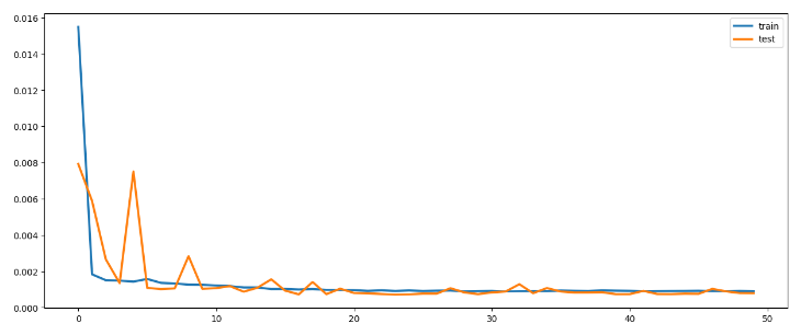

y_test_true = test[:,8]

testPredict2 = model2.predict(test_X)
testPredict2 = testPredict2.ravel()

# Inverse scaling the output, for better visual interpretation 

poll = np.array(df["pollution"])
meanop = poll.mean()
stdop = poll.std()

print(meanop, stdop)

y_test_true = y_test_true*stdop + meanop
testPredict2 = testPredict2*stdop + meanop

>>>548/548 [==============================] - 1s 1ms/step
>>>94.01351598173515 92.25122315439845

from matplotlib import pyplot as plt

plt.figure(figsize=(15,6))
plt.xlim([1000,1250])
plt.ylabel("ppm")
plt.xlabel("hrs")
plt.plot(y_test_true, c = "g", alpha = 0.90, linewidth = 2.5)
plt.plot(testPredict2, c = "darkblue", alpha = 0.75)
plt.title("Testing(Validation) data")
plt.show()

rmse = np.sqrt(mean_squared_error(y_test_true, testPredict2))
print("Test(Validation) RMSE ="  ,rmse)

>>>Test(Validation) RMSE = 2.5967174

values.shape

>>>(43799, 9)

train_x, train_y = values[:, :-1], values[:, -1]
print(train_x.shape, train_y.shape)

>>>(43799, 8) (43799,)

train_x = train_x.reshape((train_x.shape[0], 1, train_x.shape[1]))

model3 = Sequential()
model3.add(LSTM(256, input_shape=(train_x.shape[1], train_x.shape[2])))
model3.add(Dense(32))
model3.add(Dropout(0.25))
model3.add(BatchNormalization())
model3.add(Dense(1))

model3.summary()

model3.compile(loss='mse', optimizer='adam')

hist3 = model3.fit(train_x, train_y, epochs=50, batch_size=256, validation_split=0.2)

>>>Epoch 46/50
137/137 [==============================] - 1s 8ms/step - loss: 9.1802e-04 - val_loss: 6.4329e-04
Epoch 47/50
137/137 [==============================] - 1s 8ms/step - loss: 9.1274e-04 - val_loss: 6.2389e-04
Epoch 48/50
137/137 [==============================] - 1s 8ms/step - loss: 8.9003e-04 - val_loss: 6.9569e-04
Epoch 49/50
137/137 [==============================] - 1s 8ms/step - loss: 8.9664e-04 - val_loss: 6.4270e-04
Epoch 50/50
137/137 [==============================] - 1s 8ms/step - loss: 9.0767e-04 - val_loss: 6.2983e-04

plt.figure(figsize=(15,6))
plt.plot(hist3.history['loss'], label='train', linewidth = 2.5)
plt.plot(hist3.history['val_loss'], label='test',  linewidth = 2.5)
plt.legend()
plt.show()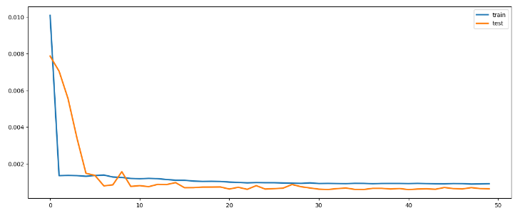

y_train_true = values[:,8]

trainPredict3 = model3.predict(train_x)
trainPredict3 = trainPredict3.ravel()

# Inverse scaling the output, for better visual interpretation 

poll = np.array(df["pollution"])
meanop = poll.mean()
stdop = poll.std()

print(meanop, stdop)

y_train_true = y_train_true*stdop + meanop
trainPredict3 = trainPredict3*stdop + meanop

>>>1369/1369 [==============================] - 2s 1ms/step
>>>94.01351598173515 92.25122315439845

from matplotlib import pyplot as plt

plt.figure(figsize=(18,5.5))
# plt.xlim([1000,1250])
plt.ylabel("ppm")
plt.xlabel("hrs")
plt.plot(y_train_true, c = "cyan", alpha = 0.90, linewidth = 2.5)
plt.plot(trainPredict3, c = "darkblue", alpha = 0.75)
plt.title("Training data")
plt.show()

# darkblue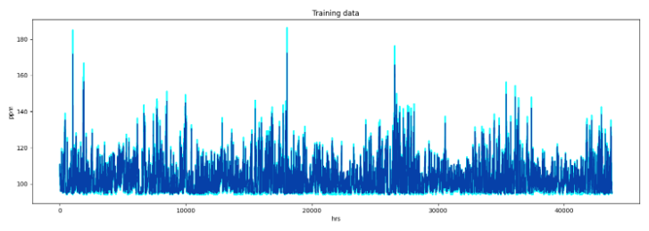

rmse = np.sqrt(mean_squared_error(y_train_true, trainPredict3))
print("Training RMSE ="  ,rmse)

>>>Training RMSE = 2.5422497

test_df = pd.read_csv("pollution_test_data1.csv")
test_df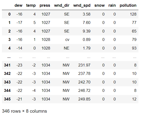

test_df["wind_dir"] = test_df["wnd_dir"].apply(func)
del test_df["wnd_dir"]

values_test = test_df.values
values_test = values_test.astype('float32')

scaler1 = MinMaxScaler()
scaled_test = scaler1.fit_transform(values_test)
reframed_test = series_to_supervised(scaled_test, 1, 1)

reframed_test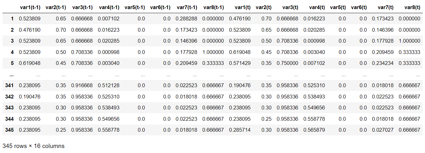

reframed_test.drop(reframed_test.columns[[9,10,11,12,13,14,15]], axis=1, inplace=True)
print(reframed_test.head())

>>>   var1(t-1)  var2(t-1)  var3(t-1)  var4(t-1)  var5(t-1)  var6(t-1)  \
1   0.523809       0.65   0.666668   0.007102        0.0        0.0   
2   0.476190       0.70   0.666668   0.016223        0.0        0.0   
3   0.523809       0.65   0.666668   0.020285        0.0        0.0   
4   0.523809       0.50   0.708336   0.000998        0.0        0.0   
5   0.619048       0.45   0.708336   0.003040        0.0        0.0   

   var7(t-1)  var8(t-1)   var1(t)  
1   0.288288   0.000000  0.476190  
2   0.173423   0.000000  0.523809  
3   0.146396   0.000000  0.523809  
4   0.177928   1.000000  0.619048  
5   0.209459   0.333333  0.571429  

values_test1 = reframed_test.values

test_x, test_y = values_test1[:, :-1], values_test1[:, -1]

test_x = test_x.reshape((test_x.shape[0], 1, test_x.shape[1]))

test_x.shape, test_y.shape

>>>((345, 1, 8), (345,))

testPredict3 = model3.predict(test_x)
testPredict3 = testPredict3.ravel()
poll = np.array(df["pollution"])
meanop = poll.mean()
stdop = poll.std()

print(meanop, stdop)

# Inverse scaling the output, for better visual interpretation 
test_y = test_y*stdop + meanop
testPredict3 = testPredict3*stdop + meanop

>>>11/11 [==============================] - 0s 880us/step
>>>94.01351598173515 92.25122315439845

from matplotlib import pyplot as plt

plt.figure(figsize=(18,5.5))
plt.ylabel("ppm")
plt.xlabel("hrs")
plt.plot(test_y, c = "lightgreen", alpha = 0.90, linewidth = 2.5)
plt.plot(testPredict3, c = "darkblue", alpha = 0.75)
plt.title("Testing data")
plt.show()
# darkblue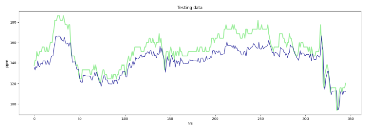

rmse = np.sqrt(mean_squared_error(test_y, testPredict3))
print("Test RMSE ="  ,rmse)

>>>Test RMSE = 11.790104