스터디노트 (DeepLearning 1)

Beginning of Deeplearning

• 뉴런 :
  - 뉴런은 입력, 가중치, 활성화함수, 출력으로 구성
  - 뉴런에서 학습할 때 변하는 것은 가중치. 처음에는 초기화를 통해 랜덤값을 넣고, 학습과정에서 일정한 값으로 수련

• 뉴런이 모여서 레이어(layer)를 구성하고, 망(net)이 된다.

• 신경망이 깊어(많아)지면 깊은 신경망 Deep Learning이 된다

Beginning of Deeplearning - Blood Fat

import numpy as np

raw_data = np.genfromtxt('./x09.txt', skip_header=36)
raw_data

from mpl_toolkits.mplot3d import Axes3D
import matplotlib.pyplot as plt
%matplotlib inline

xs = np.array(raw_data[:, 2], dtype=np.float32)
ys = np.array(raw_data[:, 3], dtype=np.float32)
zs = np.array(raw_data[:, 4], dtype=np.float32)

fig = plt.figure()
ax = fig.add_subplot(111, projection='3d')
ax.scatter(xs, ys, zs)
ax.set_xlabel('Weight')
ax.set_ylabel('Age')
ax.set_zlabel('Blood fat')
ax.view_init(15, 15)
plt.show()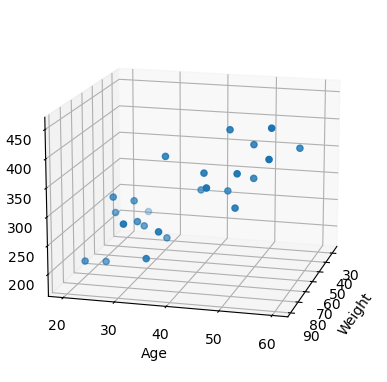

• 예제의 목적은 입력인 나이와 몸무게를 알려주면, 주어진 데이터 기준의 blood fat을 얻는 것
• 40살, 100키로인 사람의 데이터 기준 blood fat 결과가 나와야 한다
• Linear Regression
  
  
• 모델을 주어진 데이터로 얻는 것 :
  • y = xW + b.
  • 직선 모델을 얻는 것으로 하면, 주어진 입출력 데이터로 W와 b. 즉, 모델을 얻는것
• 모델을 구한 후
  • 모델(W, b)을 이용해서 질문을 하는 것. 즉, age 40, weight 80인 사람의 blood fat에 대답을 얻을 수 있다
• y = xW + b. x1, x2를 입력해서 y가 나오게 하는 weight와 bias를 구하는 것.
  
  

# 학습 대상 데이터 추리기

x_data = np.array(raw_data[:, 2:4], dtype=np.float32)
#print(x_data)
y_data = np.array(raw_data[:, 4], dtype=np.float32)
print(y_data.shape) #
y_data = y_data.reshape((25, 1))
y_data

# !pip install tensorflow

• 학습을 위해서는 loss(cost) 함수를 정해주어야 한다

• loss 함수는 간략히 말해서, 정답까지 얼마나 멀리 있는지를 측정하는 함수

• 이번에는 mse : mean square error 오차 제곱의 평균을 사용

• 옵티마이저 선정. 옵티마이저는 loss를 어떻게 줄일 것인지를 결정하는 방법을 선택하는 것.

• optimizer : loss 함수를 최소화하는 가중치를 찾아가는 과정에 대한 알고리즘

• 여기서는 rmsprop 사용
  
  

# 모델 생성
import tensorflow as tf

model = tf.keras.models.Sequential([tf.keras.layers.Dense(1, input_shape=(2, ))])
# output은 1개, 입력은 2개

model.compile(optimizer='rmsprop', loss='mse')
# rmsprop : RMSProp는 과거의 모든 기울기를 균일하게 더하지 않고 먼 과거의 기울기는 서서히 잊고 새로운 기울기 정보를 크게 반영

model.summary()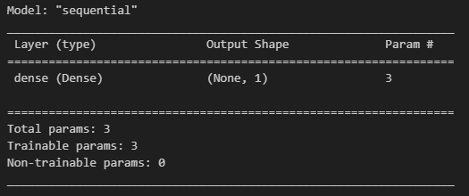

• 나이와 몸무게를 받아서 blood fat을 추정하는 모델을 학습을 통해 얻고자 함
• 모델(네트워크)을 구성했고,
• 모델의 loss function을 선정, loss의 감소를 위한 optimizer도 선정함

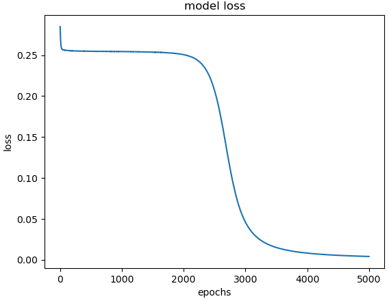
hist = model.fit(x_data, y_data, epochs=5000)

plt.plot(hist.history['loss'])
plt.title('model loss')
plt.ylabel('loss')
plt.xlabel('epochs')
plt.show()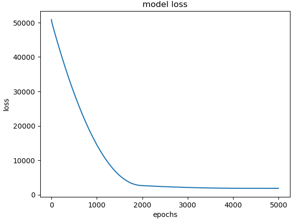

# predict

model.predict(np.array([100, 44]).reshape(1, 2))

model.predict(np.array([60, 25]).reshape(1, 2))

# 가중치, bias를 알고 싶으면

W_, b_ = model.get_weights()
print('Weight is : ', W_)
print('bias is : ', b_)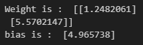

# 모델이 잘 만들어졌는지 확인하기 위해 데이터 생성

x = np.linspace(20, 100, 50).reshape(50, 1) # 나이
#print(x)
y = np.linspace(10, 70, 50).reshape(50, 1) # 몸무게
#print(y)

X = np.concatenate((x, y), axis=1) # np.concatenate : 배열 합치기
Z = np.matmul(X, W_) + b_ 
# np.matmul : 행렬곱

# 그리기

fig = plt.figure(figsize=(12, 12))
ax = fig.add_subplot(111, projection='3d')
ax.scatter(xs, ys, zs)
ax.scatter(x, y, Z)
ax.set_xlabel('Weight')
ax.set_ylabel('Age')
ax.set_zlabel('Blood fat')
ax.view_init(15, 15)
plt.show()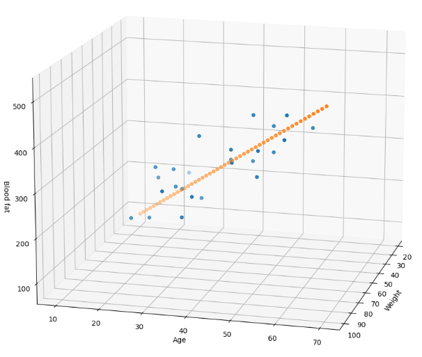

---

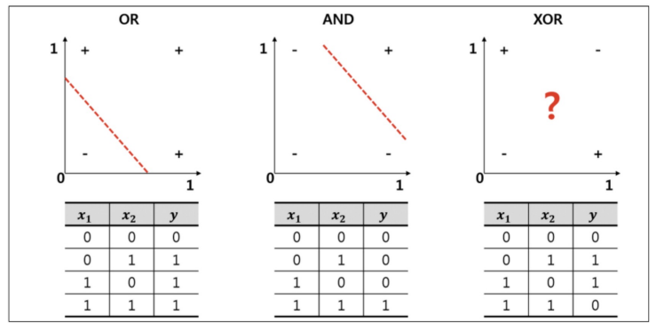
Beginning of Deeplearning - XOR

• 선형 모델로는 XOR를 풀 수 없다

  

# 데이터 준비

import numpy as np

X = np.array([[0, 0],
              [1, 0],
              [0, 1], 
              [1, 1]])
y = np.array([[0], [1], [1], [0]])

# 모델

import tensorflow as tf
from mpl_toolkits.mplot3d import Axes3D

# Dense 레이어는 입력과 출력을 모두 연결해주며, 입력과 출력을 각각 연결해주는 가중치를 포함
# 'sigmoid' : 이진분류문제, 직선이 합쳐지지 않기 위해 사용(?..)
model = tf.keras.Sequential([
    tf.keras.layers.Dense(2, activation='sigmoid', input_shape=(2, )),  
    tf.keras.layers.Dense(1, activation='sigmoid')])

• 옵티마이저를 선정하고 학습률을 선정
• loss 함수는 mse로 한다

# model.compile

model.compile(optimizer=tf.keras.optimizers.SGD(learning_rate=0.1), loss='mse')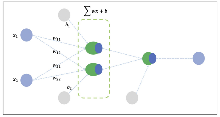

# model.summary

model.summary()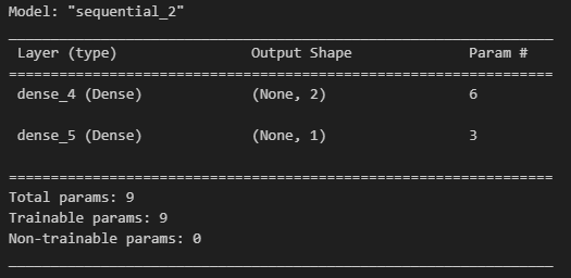

• epochs는 지정된 횟수만큼 학습하는 것
• batch_size는 한 번의 학습에 사용될 데이터의 수를 지정

hist = model.fit(X, y, epochs=5000, batch_size=1)

model.predict(X)

# loss 상황

import matplotlib.pyplot as plt
%matplotlib inline

plt.plot(hist.history['loss'])
plt.title('model loss')
plt.ylabel('loss')
plt.xlabel('epochs')
plt.show()

# 학습에서 찾은 가중치

for w in model.weights:
    print('---')
    print(w)

---

Beginning of Deeplearning - iris(분류)

• pdf 자료 꼭 같이 봐야함!

# iris 데이터

from sklearn.datasets import load_iris

iris = load_iris()

X = iris.data
y = iris.target

# 이런 모양은 특정 모델에서만 답을 잘 맞출 수 있다(?)
y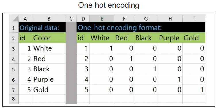

# sklearn의 one hot encoding

from sklearn.preprocessing import OneHotEncoder

enc = OneHotEncoder(sparse=False, handle_unknown='ignore')
enc.fit(y.reshape(len(y), 1))

enc.categories_

y_onehot = enc.transform(y.reshape(len(y), 1))
y_onehot

# 데이터 나누기

from sklearn.model_selection import train_test_split

X_train, X_test, y_train, y_test = train_test_split(X, y_onehot, test_size=0.2, random_state=13)

• activation : 하나의 뉴런 끝단에 activation이 붙어있다

• https://m.blog.naver.com/PostView.naver?isHttpsRedirect=true&blogId=handuelly&logNo=221824080339
  
  

• 역전파 back-propagation
  - 레이어가 여러 개가 있으면 출력단이 아닌 레이어들은 에러를 계선하기 어려운데 이걸 극복하기 위한 것
  - 내가 틀린 정도를 '미분(기울기)' 한 것.
  - 미분하고, 곱하고, 더하로를 역방향으로 반복하며 업데이트한다
  
  

• 역전파에서는 sigmoid가 문제가 있다

• gradient vanishing : 레이어가 깊을 수록 업데이트가 사라져간다. 그래서 fitting이 잘 안된다.

• ReLU : 사그라드는 sigmoid대신 죽지않는 activation func을 쓰는 것. 0 ~ 1사이로 한정짓지 않고 쭉 뻗어간다(?)

• 뉴럿넷에게 답을 회신받는 3가지 방법
  - value(얼마가 될 것같은가) : output을 그냥 받는다
  - O/X(맞나? 아닌가?) : output에 sigmoid를 적용
  - Category(종류 즁 요건이 무엇인가) : output에 softmax를 적용
  - softmax : 출력값의 확률 합을 1로 관리, 가장 높은 값을 정답이라고 말한다(?)
  
  

import tensorflow as tf

model = tf.keras.models.Sequential([
    tf.keras.layers.Dense(32, input_shape=(4, ), activation='relu'), # 입력값 32개, input_shape=(4, ) : 특성 4개 설정
    tf.keras.layers.Dense(32, activation='relu'),
    tf.keras.layers.Dense(32, activation='relu'),
    tf.keras.layers.Dense(3, activation='softmax'),]) # 출력값 3개

# adam

model.compile(optimizer='adam', loss='categorical_crossentropy',
              metrics=['accuracy'])
model.summary()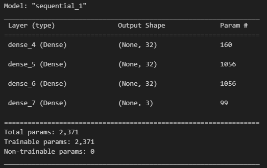

• gradient decent :

  • 기존 뉴럴넷이 가중치 parameter들을 최적화(optimize)하는 방법
  • loss function의 현 가중치에서의 기울기(gradient)를 구해서 loss를 줄이는 방향으로 업데이트

• 뉴럴넷은 loss(or cost) function을 가지고 있다. (쉽게 말하면 '틀린정도')

  • 현재 가진 weight 세팅(내 자리)에서 내가 가진 데이터를 다 넣으면 전체 에러가 계산된다
  • 거기서 미분하면 에러를 줄이는 방향을 알 수 있다(내 자리의 기울기 *반대방향)
  • 그 방향으로 정해진 스텝량(learning rate)을 곱해서 weight을 이동시킨다. 그리고 이것을 반복

• Gradient Decent :

  • 학습데이터(full-batch) 전부다 읽고나서 최적의 1스텝 간다
  • 최적인데 너무 느리다

• SGD(Stochastic Gradient Decent) :

  • 학습데이터(mini-batch, mini-batch...) 작은 토막마다 일단 1스텝 간다
  • 조금 헤매도 어쨌든 인근에 아주 빨리 간다

• 데이터가 복잡할 때는 일단 Adam을 쓰자
  
  

# 학습

hist = model.fit(X_train, y_train, epochs=100)

# test 데이터에 대한 accuracy

model.evaluate(X_test, y_test, verbose = 2)

# loss와 acc의 변화
# 주황색이 accuracy
# 파란색이 loss
import matplotlib.pyplot as plt
%matplotlib inline


plt.plot(hist.history['loss'])
plt.plot(hist.history['accuracy'])
plt.grid()
plt.title('model loss')
plt.ylabel('loss')
plt.xlabel('epochs')
plt.show()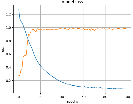

---

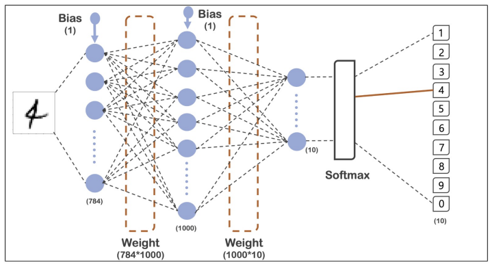
Beginning of Deeplearning - MNIST

# 데이터 읽기
# 각 픽셀이 255값이 최댓값이어서 0 ~ 1 사이의 값으로 조정(일종의 min mas scaler)

import tensorflow as tf

mnist = tf.keras.datasets.mnist

(x_train, y_train), (x_test, y_test) = mnist.load_data()
x_train, x_test = x_train / 255.0, x_test / 255.0

x_train

• one-hot-encoding
  - loss 함수를 sparse_categorical_crossentropy로 설정하면 같은 효과이다

# 모델 생성

model = tf.keras.models.Sequential([
    tf.keras.layers.Flatten(input_shape=(28, 28)), # Flatten : 일렬로 펼치는 것
    tf.keras.layers.Dense(1000, activation='relu'),
    tf.keras.layers.Dense(10, activation='softmax')
])

model.compile(optimizer='adam', 
              loss='sparse_categorical_crossentropy', 
              metrics=['accuracy'])

model.summary()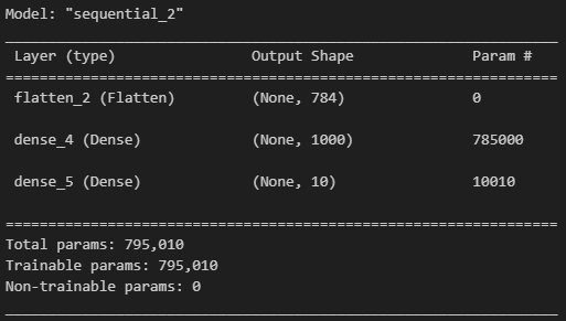

# fit
# https://m.blog.naver.com/qbxlvnf11/221449297033

import time

start_time = time.time()
hist = model.fit(x_train, y_train, validation_data=(x_test, y_test),
                 epochs=10, batch_size=100, verbose=1)

print('Fit time : ', time.time() - start_time)

# acc, loss

import matplotlib.pyplot as plt

%matplotlib inline

plot_target = ['loss', 'val_loss', 'accuracy', 'val_accuracy']

plt.figure(figsize=(12, 8))

for each in plot_target:
    plt.plot(hist.history[each], label = each)

plt.legend()
plt.grid()
plt.show()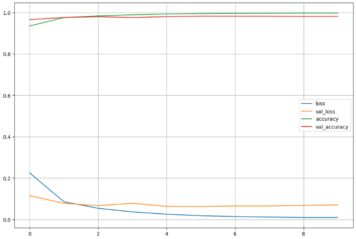

score = model.evaluate(x_test, y_test)
print('Test loss : ', score[0])
print('Test accuracy : ', score[1])

# 뭐가 틀렸는지 확인

import numpy as np

predicted_result = model.predict(x_test)
predicted_result[0]

predicted_labels = np.argmax(predicted_result, axis=1) # argmax : 최대값의 인덱스를 가져와 읽음
predicted_labels[:10]

y_test[:10]

# 틀린 데이터의 인덱스만 모으기

wrong_result = []

for n in range(0, len(y_test)):
    if predicted_labels[n] != y_test[n]:
        wrong_result.append(n)

len(wrong_result)

# 그중 16개만

import random

samples = random.choices(population=wrong_result, k=16)
samples

# 뭘 틀렸는지 확인

plt.figure(figsize=(14, 12))

for idx, n in enumerate(samples):
    plt.subplot(4, 4, idx+1)
    plt.imshow(x_test[n].reshape(28, 28), cmap='Greys', interpolation='nearest')
    plt.title('Label : ' + str(y_test[n]) + ' Predict : '+str(predicted_labels[n]))
    plt.axis('off')

plt.show()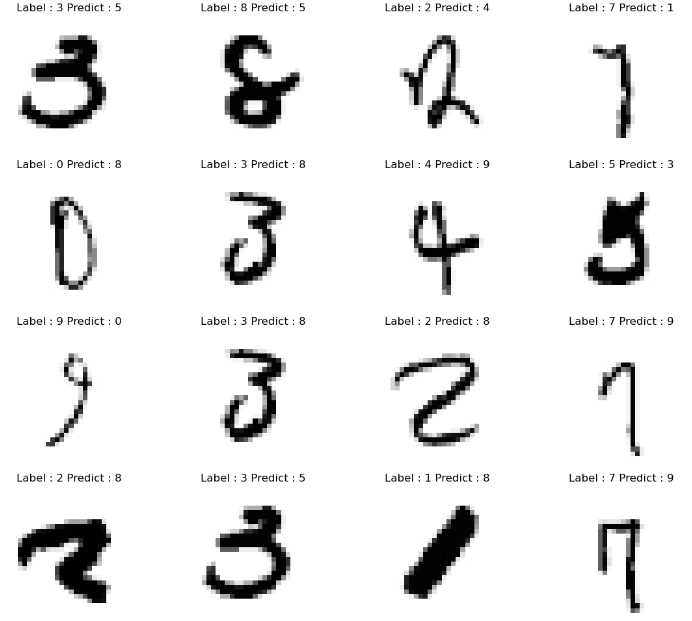

---

Beginning of Deeplearning - MNIST fashion data

• 숫자로 된 MNIST 데이터처럼 28*28 크기의 패션과 관련된 10개 종류의 데이터

# 데이터 읽기

import tensorflow as tf

fashion_mnist = tf.keras.datasets.fashion_mnist

(X_train, y_train), (X_test, y_test) = fashion_mnist.load_data()
X_train, X_test = X_train / 255.0, X_test / 255.0

# 어떻게 생겼는지 확인

import random
import matplotlib.pyplot as plt


%matplotlib inline

samples = random.choices(population=range(0, len(y_train)), k=16)
samples

plt.figure(figsize=(14, 12))

for idx, n in enumerate(samples):
    plt.subplot(4, 4, idx + 1)
    plt.imshow(X_train[n].reshape(28, 28), cmap='Greys', interpolation='nearest')
    plt.title('Label : ' + str(y_train[n]))
    plt.axis('off')

plt.show()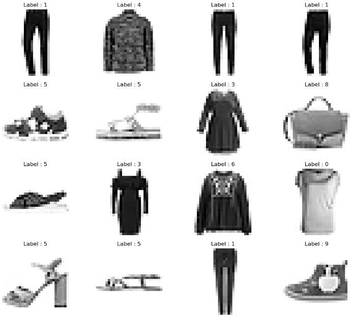

# 모델은 숫자 때와 동일한 구조로 두기

model = tf.keras.models.Sequential([
    tf.keras.layers.Flatten(input_shape=(28, 28)),
    tf.keras.layers.Dense(1000, activation='relu'),
    tf.keras.layers.Dense(10, activation='softmax')
])

model.compile(optimizer='adam', 
              loss='sparse_categorical_crossentropy',
              metrics=['accuracy'])

model.summary()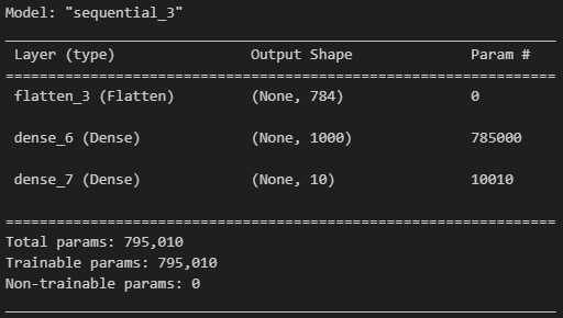

# fit

import time

start_time = time.time()
hist = model.fit(X_train, y_train, validation_data=(X_test, y_test),
                 epochs=10, batch_size=100, verbose=1)
print('Fit time : ', time.time() - start_time)

# 학습 상황 관찰

import matplotlib.pyplot as plt
%matplotlib inline

# val_loss와 train loss 사이에 간격 발생

plot_target = ['loss', 'val_loss', 'accuracy', 'val_accuracy']

plt.figure(figsize=(12, 8))

for each in plot_target:
    plt.plot(hist.history[each], label=each)

plt.legend()
plt.grid()
plt.show()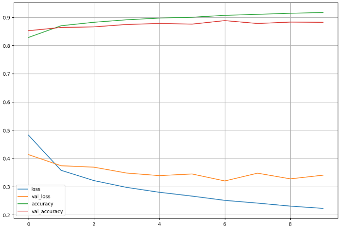

# 테스트 데이터 accuracy

score = model.evaluate(X_test, y_test)
print('Test loss : ', score[0])
print('Test accuracy : ', score[1])

# 어떤 데이터가 틀렸는지 추출

import numpy as np

predicted_result = model.predict(X_test)
predicted_labels = np.argmax(predicted_result, axis=1)
predicted_labels[:10]

y_test[:10]

# 틀린 데이터 모으기

wrong_result = []

for n in range(0, len(y_test)):
    if predicted_labels[n] != y_test[n]:
        wrong_result.append(n)

len(wrong_result)

# 16개만 선택해서 그리기

import random

samples = random.choices(population=wrong_result, k=16)
samples

plt.figure(figsize=(14, 12))

for idx, n in enumerate(samples):
    plt.subplot(4, 4, idx + 1)
    plt.imshow(X_test[n].reshape(28, 28), cmap='Greys', interpolation='nearest')
    plt.title('Label : ' + str(y_test[n]) + ' Predict : '+str(predicted_labels[n]))
    plt.axis('off')

plt.show()


# 0 : 티셔츠, 1 : 바지, 2: 스웨터, 3 : 드레스, 4 : 코트, 5 : 샌들, 6 : 셔츠, 7 : 운동화, 8 : 가방, 9 : 부츠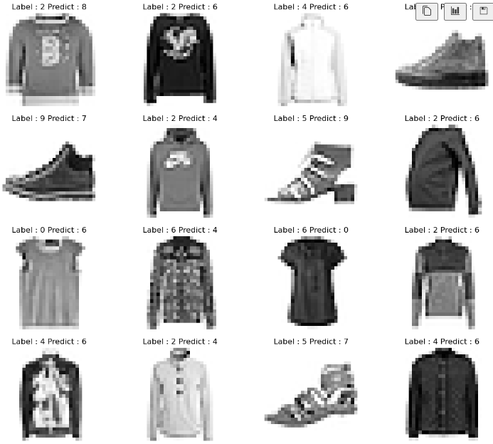

---

Beginning of Deeplearning - CNN

• Convolutional Filter : 학습을 통해 필터도 구할 수 있다

• Convolution : 특정 패턴이 있는지 박스로 훓으며 마킹.

• Convolution 박스로 밀고나면, 숫자가 나온다. 그 숫자를 Activation(주로 ReLU)에 넣어 나온 값으로 이미지 지도를 새로 그린다

• CNN : 사진에서 특징을 검출하는 기능을 가진 레이어가 있다(?..)

• 풀링 : 사진의 사이즈를 줄이는 것(?..)

• MaxPooling : 사이즈를 점진적으로 줄이는 법. n*n(Pool)을 중요한 정보(Max) 한개로 줄인다. 선명한 정보만 남겨서, 판단과 학습이 쉬워지고 노이즈가 줄면서, 덤으로 융통성도 확보된다.

  • stride : 몇 칸을 건너갈 것인가

• Conv Layer : 패턴들을 쌓아가며 점차 복잡한 패턴을 인식한다(Conv). 사이즈를 줄여가며, 더욱 추상화해나간다(maxpooling)

• Zero padding : (padding = 'same')사이즈 유지를 위해 conv 전에 0을 모서리에 보내고 한다

• dropout : 과적합 방지, 학습 시킬 때, 일부러 저오를 누락시키거나, 중간중간 노드를 끈다

MNIST

# 데이터 정리

from tensorflow.keras import datasets

mnist = datasets.mnist

(X_train, y_train), (X_test, y_test) = mnist.load_data()
X_train, X_test = X_train / 255.0, X_test / 255.0

X_train = X_train.reshape((60000, 28, 28, 1))
X_test = X_test.reshape((10000, 28, 28, 1))

# 모델 구성
# 어렵다..

from tensorflow.keras import layers, models

model = models.Sequential([
    layers.Conv2D(32, kernel_size = (5, 5), strides=(1, 1),
                  padding='same', activation='relu', input_shape=(28, 28, 1)),
    layers.MaxPooling2D(pool_size=(2, 2), strides = (2, 2)),
    layers.Conv2D(64, (2, 2), activation='relu', padding='same'),
    layers.MaxPooling2D(pool_size=(2, 2)),
    layers.Dropout(0.25),
    layers.Flatten(),
    layers.Dense(1000, activation='relu'),
    layers.Dense(10, activation='softmax')
])

model.summary()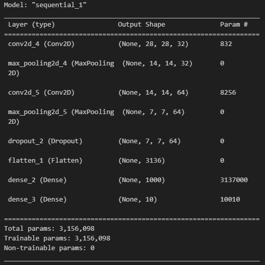

# 훈련

import time

model.compile(optimizer='adam', loss='sparse_categorical_crossentropy', metrics=['accuracy'])

start_time = time.time()
hist = model.fit(X_train, y_train, epochs=5, verbose=1,
                 validation_data = (X_test, y_test))

print('fit time : ', time.time() - start_time)

# 훈련 상황

import matplotlib.pyplot as plt
%matplotlib inline

plot_target = ['loss', 'val_loss', 'accuracy', 'val_accuracy']
plt.figure(figsize=(12, 8))

for each in plot_target:
    plt.plot(hist.history[each], label=each)

plt.legend()
plt.grid()
plt.show()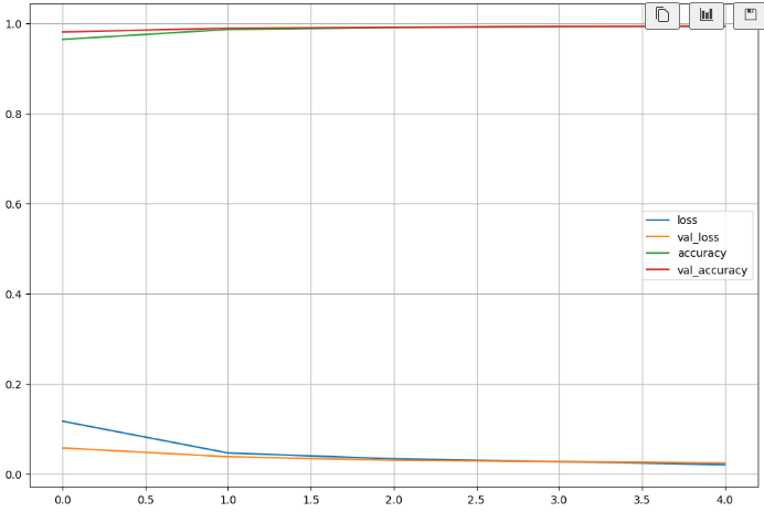

# Test Accuracy 99%

score = model.evaluate(X_test, y_test)
print('Test loss : ', score[0])
print('Test accuray : ', score[1])

# 틀린 데이터 찾기

import numpy as np

predicted_result = model.predict(X_test)
predicted_labels = np.argmax(predicted_result, axis=1)
predicted_labels[:10]

# 틀린 데이터 모으기

wrong_result = []

for n in range(0, len(y_test)):
    if predicted_labels[n] != y_test[n]:
        wrong_result.append(n)

len(wrong_result)

# 틀린 것 중 16개

import random

samples = random.choices(population=wrong_result, k=16)
samples

plt.figure(figsize=(14, 12))

for idx, n in enumerate(samples):
    plt.subplot(4, 4, idx + 1)
    plt.imshow(X_test[n].reshape(28, 28), cmap='Greys', interpolation='nearest')
    plt.title('Label : '+str(y_test[n])+' Predict : '+str(predicted_labels[n]))
    plt.axis('off')

plt.show()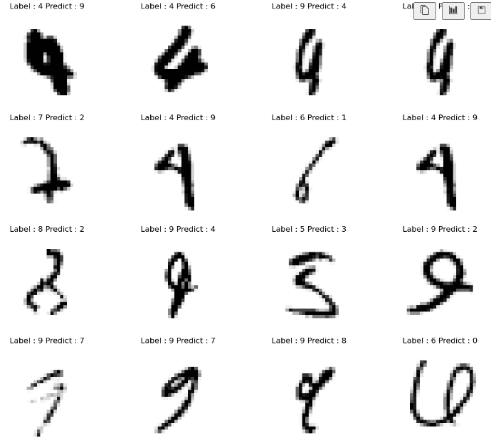

# 모델 저장

model.save('MNIST_CNN_model.h5')

---

MNIST fasion

from tensorflow.keras import datasets

mnist = datasets.fashion_mnist

(X_train, y_train), (X_test, y_test) = mnist.load_data()
X_train, X_test = X_train / 255.0, X_test / 255.0

X_train = X_train.reshape((60000, 28, 28, 1))
X_test = X_test.reshape((10000, 28, 28, 1))

# 모델 구성

from tensorflow.keras import layers, models

model = models.Sequential([
    layers.Conv2D(32, kernel_size = (5, 5), strides=(1, 1),
                  padding='same', activation='relu', input_shape=(28, 28, 1)),
    layers.MaxPooling2D(pool_size=(2, 2), strides = (2, 2)),
    layers.Conv2D(64, (2, 2), activation='relu', padding='same'),
    layers.MaxPooling2D(pool_size=(2, 2)),
    layers.Dropout(0.25),
    layers.Flatten(),
    layers.Dense(1000, activation='relu'),
    layers.Dense(10, activation='softmax')
])

model.summary()

# 훈련

import time

model.compile(optimizer='adam', loss='sparse_categorical_crossentropy', metrics=['accuracy'])

start_time = time.time()
hist = model.fit(X_train, y_train, epochs=5, verbose=1,
                 validation_data = (X_test, y_test))

print('fit time : ', time.time() - start_time)

# 훈련 상황

import matplotlib.pyplot as plt
%matplotlib inline

plot_target = ['loss', 'val_loss', 'accuracy', 'val_accuracy']
plt.figure(figsize=(12, 8))

for each in plot_target:
    plt.plot(hist.history[each], label=each)

plt.legend()
plt.grid()
plt.show()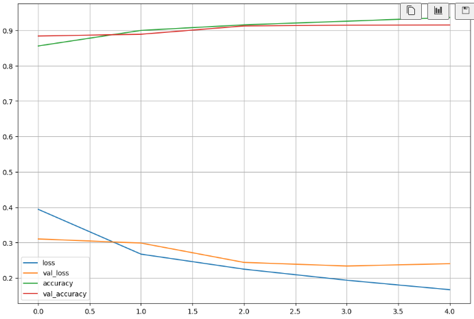

# test accuracy가 91%

score = model.evaluate(X_test, y_test)
print('Test loss : ', score[0])
print('Test accuracy : ', score[1])

어렵다..자료 참고해서 봐야함

💻 출처 : 제로베이스 데이터 취업 스쿨