machine learning - Logistic Regression, Ensemble : 데이터 취업 스쿨 스터디 노트 1/22

✨데이터 자체에 집중하고 데이터에서 답을 얻으려고 노력해야지
모델에서 마법처럼 성능 향상이 일어나는 경우는 드물다.

1. Logistic Regression

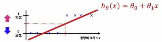
Linear Regression을 그대로 적용하면 분류 문제를 해결하기 어렵다.
예측값이 0보다 작거나 1보다 큰 값을 가질 수 있기 때문이다.
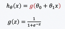
예측값이 항상 0에서 1 사이의 값을 갖도록 Hypothesis 함수를 수정하자!

import numpy as np
import matplotlib.pyplot as plt
%matplotlib inline

z = np.arange(-10, 10, 0.01)
g = 1 / (1+np.exp(-z))

plt.figure(figsize=(12, 8))
# gca() : 설정값을 변경할 수 있는 함수
ax = plt.gca()

ax.plot(z, g)
# spines : 축 설정
ax.spines['left'].set_position('zero')
ax.spines['bottom'].set_position('center')
ax.spines['right'].set_color('none')
ax.spines['top'].set_color('none')

plt.show()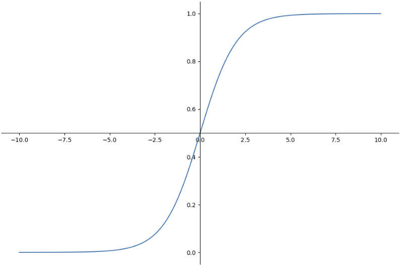

시그모이드 함수에 직선의 함수를 넣어서 결과를 판정한다.
예측값 = 주어진 x(종양의 크기)에서의 예측 결과가 1(악성)이 될 확률

Decision Boundary

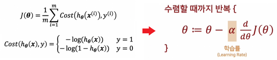
Linear Regression에서 Cost Function은 단순하지만, Logistic Regression의 미분식은 복잡하기 때문에 Cost Function을 재정의할 필요가 있다.

h = np.arange(0.01, 1, 0.01)

C0 = -np.log(1-h)
C1 = -np.log(h)

plt.figure(figsize=(12, 8))
plt.plot(h, C0, label='y=0')
plt.plot(h, C1, label='y=1')
plt.legend()
plt.show()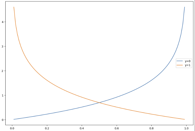

2. 실습 : wine data

from sklearn.linear_model import LogisticRegression
from sklearn.metrics import accuracy_score

# solver : 최적합 알고리즘 선택
# 데이터 수가 작으면 주로 liblinear
lr = LogisticRegression(solver='liblinear', random_state=13)
lr.fit(X_train, y_train)

y_pred_tr = lr.predict(X_train)
y_pred_test = lr.predict(X_test)

accuracy_score(y_train, y_pred_tr), accuracy_score(y_test, y_pred_test)

>>>
(0.7427361939580527, 0.7438461538461538)

StandardScaler 적용해서 비교해보면 (+Pipeline)

from sklearn.pipeline import Pipeline
from sklearn.preprocessing import StandardScaler

estimators = [('scaler', StandardScaler()),
               ('clf', LogisticRegression(solver='liblinear', random_state=13))]
pipe = Pipeline(estimators)

pipe.fit(X_train, y_train)
y_pred_tr = pipe.predict(X_train)
y_pred_test = pipe.predict(X_test)

accuracy_score(y_train, y_pred_tr), accuracy_score(y_test, y_pred_test)

>>>
(0.7444679622859341, 0.7469230769230769)

모델 간 비교를 위해 DecisionTreeClassifier 적용

from sklearn.tree import DecisionTreeClassifier

wine_tree = DecisionTreeClassifier(max_depth=2, random_state=13)
wine_tree.fit(X_train, y_train)

# AUC 그래프를 통한 모델 간 비교
from sklearn.metrics import roc_curve

models = {
    'logistic regression': pipe,
    'decision tree': wine_tree
}

plt.figure(figsize=(10, 8))
plt.plot([0, 1], [0, 1]) # 기준선

for model_name, model in models.items():
  pred = model.predict_proba(X_test)[:, 1]
  fpr, tpr, thresholds = roc_curve(y_test, pred)
  plt.plot(fpr, tpr, label=model_name)

plt.grid()
plt.legend()
plt.show()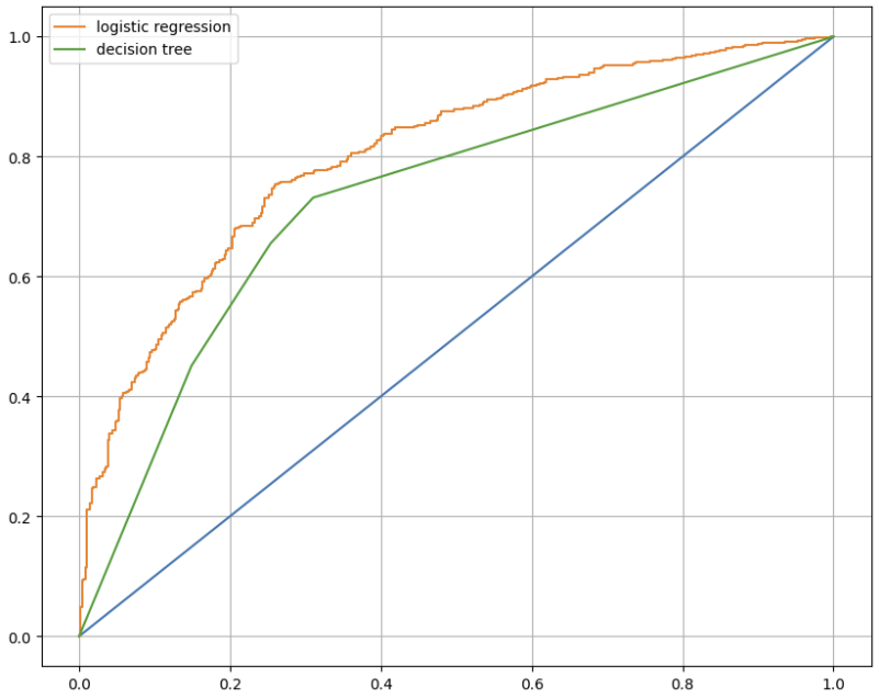

3. 실습 : PIMA 인디언 당뇨병 예측

# 모든 컬럼이 int, float ➡ 혹시 모르니 모두 float로 변경
pima = pima.astype('float')

# 상관관계 확인
import seaborn as sns

plt.figure(figsize=(12, 10))
sns.heatmap(pima.corr(), cmap='YlGnBu')
plt.show()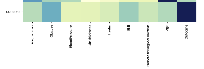

# 결측치 확인
(pima == 0).astype(int).sum()

>>>
Pregnancies                 111
Glucose                       5
BloodPressure                35
SkinThickness               227
Insulin                     374
BMI                          11
DiabetesPedigreeFunction      0
Age                           0
Outcome                     500

결측치는 데이터에 따라 그 정의가 다르다. 예를 들어 혈압이 0일 수는 없다.
PIMA 인디언에 대한 정보와 의학적 지식이 부족하므로 결측치를 평균값으로 대체한다.

zero_features = ['Glucose', 'BloodPressure', 'SkinThickness', 'BMI']
pima[zero_features] = pima[zero_features].replace(0, pima[zero_features].mean())

X = pima.drop(['Outcome'], axis=1)
y = pima['Outcome']

X_train, X_test, y_train, y_test = train_test_split(X, y, test_size=0.2,
                                                    random_state=13, stratify=y)
                                                    
estimators = [('scaler', StandardScaler()),
               ('clf', LogisticRegression(solver='liblinear', random_state=13))]
pipe_lr = Pipeline(estimators)
pipe_lr.fit(X_train, y_train)
pred = pipe_lr.predict(X_test)

from sklearn.metrics import (accuracy_score, recall_score, precision_score,
                             roc_auc_score, f1_score)

print(accuracy_score(y_test, pred))
print(recall_score(y_test, pred))
print(precision_score(y_test, pred))
print(roc_auc_score(y_test, pred))
print(f1_score(y_test, pred))

>>>
0.7727272727272727
0.6111111111111112
0.7021276595744681
0.7355555555555556
0.6534653465346535

다변수 방정식의 계수 값 확인하기

coeff = list(pipe_lr['clf'].coef_[0])
labels = list(X_train.columns)

features = pd.DataFrame({'Features': labels, 'importance': coeff})
features.sort_values(by=['importance'], ascending=True, inplace=True)
features['positive'] = features['importance'] > 0
features.set_index('Features', inplace=True)

features['importance'].plot(kind='barh', figsize=(11, 6),
                            color=features['positive'].map({True: 'blue', False: 'red'}))
plt.xlabel('Importance')
plt.show()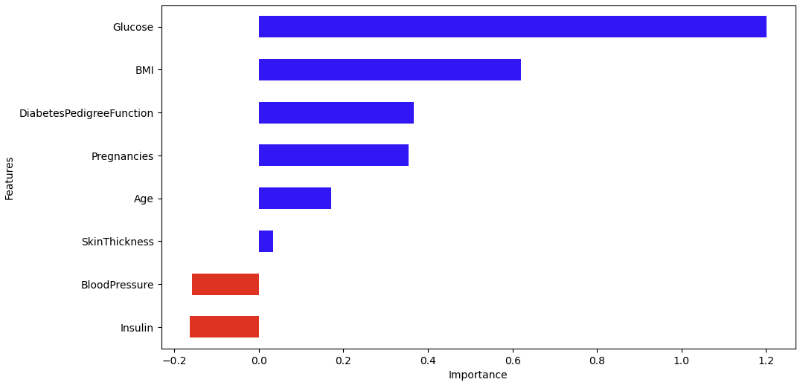

4. 정밀도와 재현율의 trade-off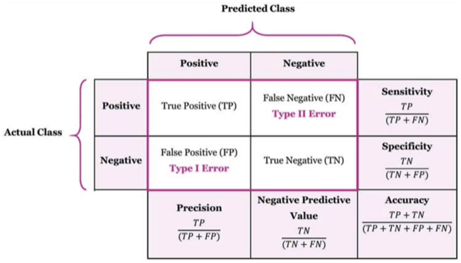

thresholds로 정밀도와 재현율을 바꿀 수 있지만, 이것이 모델의 성능을 향상시키지는 않는다. 더 많은 데이터가 들어올 때 작은 thresholds의 움직임은 큰 변화를 주지 않고, thresholds를 극단적으로 바꾸는 것도 좋지 않다. ➡ 잘 사용하지 않으나 방법을 알고 있자!

앞서 실습한 wine 데이터를 이용했다.

from sklearn.metrics import classification_report

print(classification_report(y_test, lr.predict(X_test)))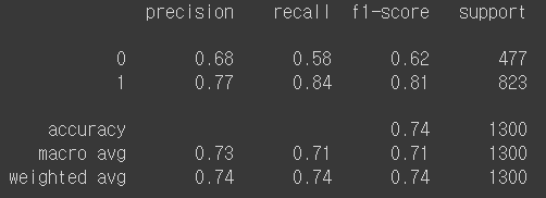

• quality > 5 ➡ 1
• precision(1) : 1이라고 예측한 것 중에서 1인 확률
• recall(1) : 실제 1인 것 중에서 1이라고 예측한 확률
• support : 개수
• macro avg : 클래스별 평균
• weighted avg : 클래스별 가중평균

from sklearn.metrics import confusion_matrix

confusion_matrix(y_test, lr.predict(X_test))

>>>
array([[275, 202],
       [131, 692]])

from sklearn.metrics import precision_recall_curve

pred = lr.predict_proba(X_test)[:, 1]
precisions, recalls, thresholds = precision_recall_curve(y_test, pred)

plt.figure(figsize=(10, 8))
# thresholds의 크기만큼만
plt.plot(thresholds, precisions[:len(thresholds)], label='precision')
plt.plot(thresholds, recalls[:len(thresholds)], label='recall')
plt.grid()
plt.legend()
plt.show()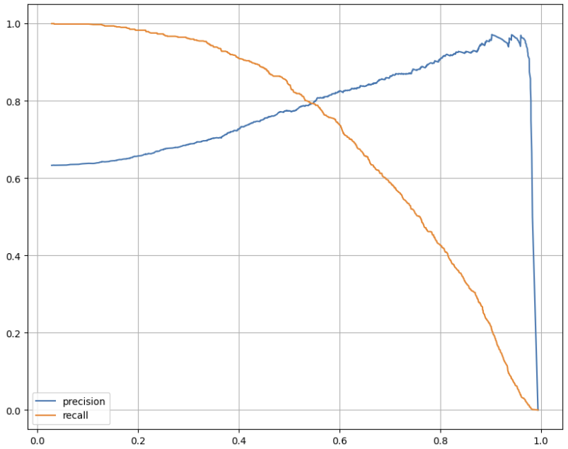

threshold 변경하기

# predict() ➡ threshold=0.5
pred_predict = lr.predict(X_test)
pred_predict

>>>
array([1, 0, 1, ..., 1, 0, 1])

pred_proba = lr.predict_proba(X_test)
pred_proba

>>>
array([[0.40537064, 0.59462936],
       [0.51023887, 0.48976113],
       [0.10180603, 0.89819397],
       ...,
       [0.22538943, 0.77461057],
       [0.67355628, 0.32644372],
       [0.31430379, 0.68569621]])

from sklearn.preprocessing import Binarizer

binarizer = Binarizer(threshold=0.6).fit(pred_proba)
pred_bin = binarizer.transform(pred_proba)[:, 1]
pred_bin

>>>
array([0., 0., 1., ..., 1., 0., 1.])

print(classification_report(y_test, pred_bin))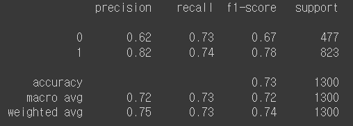

이전 결과(threshold=0.5)와 비교해보자.

5. 앙상블 기법

여러 개의 분류기를 생성하고 그 예측을 결합하여 최종 예측을 하는 방법

5-1. Voting & Bagging

Bagging : 데이터를 중복을 허용하여 샘플링하고(Bootstrapping) 각각의 데이터에 같은 알고리즘을 적용

5-2. Soft Voting & Hard Voting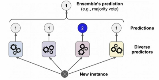

Soft Voting : 1과 2의 확률의 평균을 각각 구해서 비교한다.
Hard Voting : 다수결의 원칙과 비슷하다. 2를 제외한다.

5-3. 랜덤포레스트(Random Forest)

• 대표적인 Bagging 방법
• 부트스트래핑으로 샘플링된 각각의 데이터에 결정나무 알고리즘을 적용하여 얻은 결과를 소프트보팅하여 최종 결과를 얻음
• 앙상블 기법 중에서 비교적 속도가 빠르고, 다양한 영역에서 높은 성능을 보여줌

6. 실습 : UCI HAR(Human Activity Recognition)

• 머신러닝을 통한 행동인식연구 : 센서신호 ➡ 특징추출 ➡ 모델학습 ➡ 행동추론
• 허리에 스마트폰을 장착한 사람들의 행동을 관찰한 데이터
• 시간 영역 데이터를 머신러닝에 적용하기 위해 여러 통계적 데이터로 변환함
• 시간 영역의 평균/분산/피크/중간 값, 주파수 영역의 평균/분산 등으로 변환한 수치

6-1. 데이터 가져오기

feature_name_df = pd.read_csv(url, sep='\s+',
                              names=['column_index', 'column_name'])
feature_name_df.head()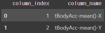

feature_name_df.info()

>>>
 0   column_index  561 non-null    int64 
 1   column_name   561 non-null    object

feature_name = feature_name_df.iloc[:, 1].values.tolist()

X_train = pd.read_csv(X_train_url, sep='\s+', header=None)
X_test = pd.read_csv(X_test_url, sep='\s+', header=None)

X_train.columns = feature_name
X_test.columns = feature_name

y_train = pd.read_csv(y_train_url, sep='\s+', header=None, names=['action'])
y_test = pd.read_csv(y_test_url, sep='\s+', header=None, names=['action'])

X_train.shape, X_test.shape, y_train.shape, y_test.shape

>>>
((7352, 561), (2947, 561), (7352, 1), (2947, 1))

y_train['action'].value_counts()

>>>
6    1407
5    1374
4    1286
1    1226
2    1073
3     986

6-2. 결정나무 적용

dt_clf = DecisionTreeClassifier(random_state=13, max_depth=4)
dt_clf.fit(X_train, y_train)
pred = dt_clf.predict(X_test)
accuracy_score(y_test, pred)

GridSearchCV를 이용하여 max_depth 다양하게 지정하기

from sklearn.model_selection import GridSearchCV

params = {
    'max_depth': [6, 8, 10, 12, 16, 20, 24]
}
grid_cv = GridSearchCV(dt_clf, param_grid=params, scoring='accuracy',
                       cv=5, return_train_score=True)
grid_cv.fit(X_train, y_train)

grid_cv.best_score_, grid_cv.best_params_

>>>
(0.8543335321892183, {'max_depth': 8})

cv_results_df = pd.DataFrame(grid_cv.cv_results_)
cv_results_df[['param_max_depth', 'mean_test_score', 'mean_train_score']]

>>>
	param_max_depth		mean_test_score		mean_train_score
0	6					0.843444			0.944879
1	8					0.854334			0.982692
2	10					0.847125			0.993369
3	12					0.841958			0.997212
4	16					0.841958			0.999660
5	20					0.842365			0.999966
6	24					0.841821			1.000000

train과 test의 score 차이가 있다는 점을 주의하자.

# test 데이터 예측
max_depth = [6, 8, 10, 12, 16, 20, 24]
for depth in max_depth:
  dt_clf = DecisionTreeClassifier(max_depth=depth, random_state=13)
  dt_clf.fit(X_train, y_train)

  pred = dt_clf.predict(X_test)
  accuracy = accuracy_score(y_test, pred)

  print(f'Max_depth={depth}, Accuracy={accuracy}')
  
>>>
Max_depth=6, Accuracy=0.8554462164913471
Max_depth=8, Accuracy=0.8734306073973532
Max_depth=10, Accuracy=0.8615541228367831
Max_depth=12, Accuracy=0.8595181540549711
Max_depth=16, Accuracy=0.8669833729216152
Max_depth=20, Accuracy=0.8652867322701052
Max_depth=24, Accuracy=0.8652867322701052

test 데이터로 성능을 확인해봐도 Max_depth=8이 가장 좋다.

best_dt_clf = grid_cv.best_estimator_
pred1 = best_dt_clf.predict(X_test)
accuracy_score(y_test, pred1)

>>>
0.8734306073973532

이렇게해도 같은 값을 얻을 수 있다.

6-3. 랜덤포레스트 적용

from sklearn.ensemble import RandomForestClassifier

params = {
    'max_depth': [6, 8, 10],
    'n_estimators': [50, 100, 200], # 나무 몇 그루 사용
    'min_samples_leaf': [8, 12], # 맨 끝에 오는 leaf의 수
    'min_samples_split': [8, 12]  # 분할 기준에서 최소한으로 남는 데이터 수
}

rf_clf = RandomForestClassifier(random_state=13, n_jobs=-1) # n_jobs=-1 코어 다 사용
grid_cv = GridSearchCV(rf_clf, param_grid=params, cv=2, n_jobs=-1)
grid_cv.fit(X_train, y_train)

cv_results_df = pd.DataFrame(grid_cv.cv_results_)
target_cols = ['rank_test_score', 'mean_test_score', 'param_n_estimators', 'param_max_depth']
cv_results_df[target_cols].sort_values('rank_test_score').head()

>>>
	rank_test_score	mean_test_score	param_n_estimators	param_max_depth
28	1				0.915125		100					10
25	1				0.915125		100					10
23	3				0.912813		200					8
20	3				0.912813		200					8
35	5				0.912541		200					10

grid_cv.best_estimator_

>>>
RandomForestClassifier(max_depth=10, min_samples_leaf=8, min_samples_split=8,
                       n_jobs=-1, random_state=13)

rf_clf_best = grid_cv.best_estimator_
rf_clf_best.fit(X_train, y_train)

pred1 = rf_clf_best.predict(X_test)
accuracy_score(y_test, pred1)

>>>
0.9205972175093315

6-4. 데이터 중요 특성 추출

best_cols_values = rf_clf_best.feature_importances_
best_cols = pd.Series(best_cols_values, index=X_train.columns)
top20_cols = best_cols.sort_values(ascending=False)[:20]
top20_cols

import seaborn as sns

plt.figure(figsize=(8, 8))
sns.barplot(x=top20_cols, y=top20_cols.index)
plt.show()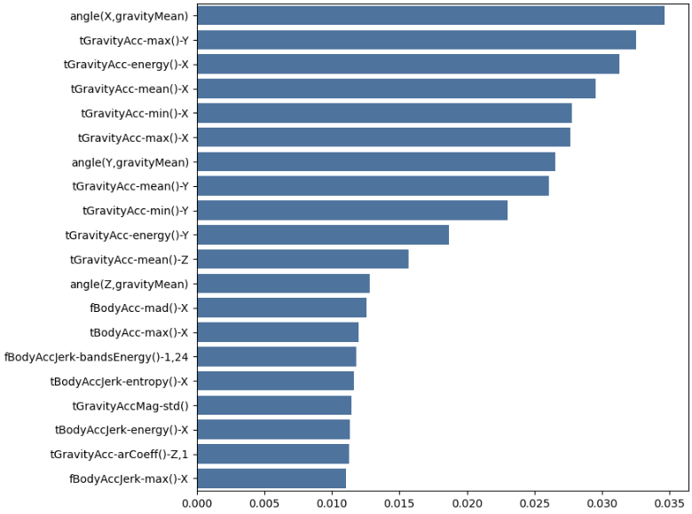

X_train_re = X_train[top20_cols.index]
X_test_re = X_test[top20_cols.index]

rf_clf_best_re = grid_cv.best_estimator_
rf_clf_best_re.fit(X_train_re, y_train.values.reshape(-1, ))

pred1_re = rf_clf_best_re.predict(X_test_re)
accuracy_score(y_test, pred1_re)

561개 특성 중에서 20개 특성만 가지고 성능 확인해봐도 성능이 크게 나쁘지 않다.
상황에 맞게 선택하면 된다.