1. Basic of Regression
- 입력 변수(특징)가 하나인 경우, 선형 회귀 문제는 주어진 학습 데이터와 가장 잘 맞는 Hypothesis 함수 h를 찾는 문제가 된다.
- Hypothesis h의 파라미터 θ0, θ1를 어떻게 찾을까?
1-1. OLS(Ordinary Linear Least Square)
!pip install statsmodelsimport pandas as pd
data = {'x': [1., 2., 3., 4., 5.], 'y': [1., 3., 4., 6., 5.,]}
df = pd.DataFrame(data)
dfimport statsmodels.formula.api as smf
# 'y ~ x' = y = ax + b
lm_model = smf.ols(formula='y ~ x', data=df).fit()
lm_model.params
>>>
Intercept 0.5
x 1.1import matplotlib.pyplot as plt
import seaborn as sns
%matplotlib inline
plt.figure(figsize=(12, 10))
sns.lmplot(x='x', y='y', data=df)
plt.xlim([0, 5])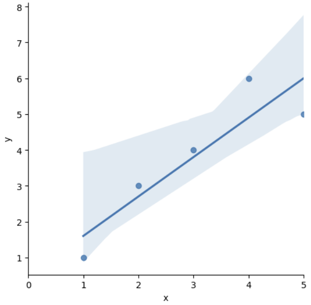
1-2. 잔차 평가(Residue)
- 잔차의 평균이 0이고 정규분포를 따르는지 확인하는 것
- 잔차는 평균이 0인 정규분포를 따라야 함 ➡ 그래서 회귀한다는 표현을 사용
resid = lm_model.resid
resid

>>>
0   -0.6
1    0.3
2    0.2
3    1.1
4   -1.0
1-3. 결정계수 (R-Squared)
import numpy as np

# df['y'] = df.y
mu = np.mean(df['y'])
y = df['y']
yhat = lm_model.predict()
np.sum((yhat - mu)**2 / np.sum((y - mu)**2)) # 0.8175675675675682
lm_model.rsquared # 0.8175675675675674# sns.distplot(resid, color='black')
sns.histplot(resid, kde=True, stat="density", kde_kws=dict(cut=3),
bins=3, alpha=.4, edgecolor=(1, 1, 1, .4), color='black')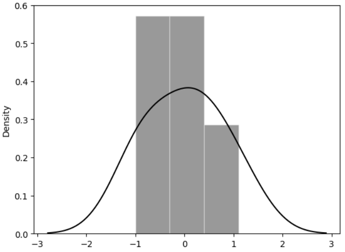
2. 통계적 회귀
3. Cost Function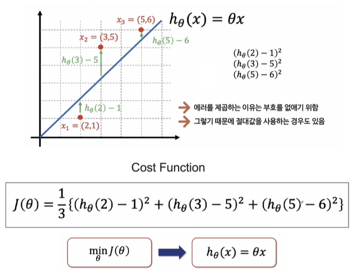
Cost Function은 에러를 표현하는 도구이다.
Cost Function을 최소화할 수 있다면 최적의 직선을 찾을 수 있다.
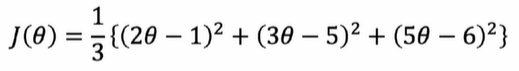
3-1. 손으로 풀기
# 숫자를 간결하게 하기 위해 3으로 나누지 않음
np.poly1d([2, -1])**2 + np.poly1d([3, -5])**2 + np.poly1d([5, -6])**2
# 모듈 설치
!pip install sympy
import sympy as sym
theta = sym.Symbol('theta')
diff_th = sym.diff(38*theta**2 - 94*theta + 62, theta) # 미분
diff_th
>>>
76θ−94θ는 대략 1.23이 나온다.
※ poly1d
Numpy의 polyfit과 poly1d의 사용법 - 최소제곱법과 polynomial class
import numpy as np

a = np.poly1d([1, 1])  # (x + 1)
b = np.poly1d([1, -1]) # (x - 1)
a * b # (x + 1)(x - 1)

>>
poly1d([ 1,  0, -1])
3-2. Gradient Descent
- 앞의 문제와 달리, 현실의 문제는 복잡하여 입력 데이터가 여러 개일 때가 많다.
- 데이터의 특징(feature)이 여러 개라면 평면상의 방정식이 아니라 다차원에서 고민해야 한다.
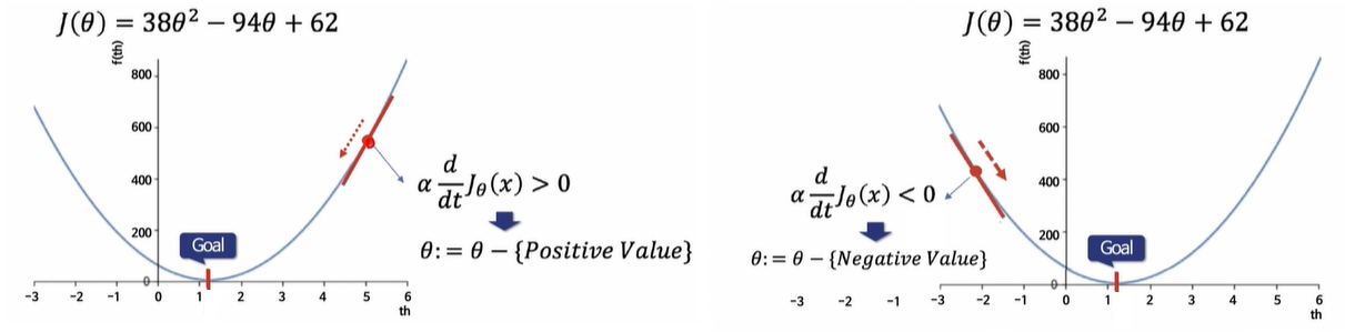
- Gradient Descent : 미분을 해서 어떤 방향으로 가야할지 정하는 것
- 학습률(α, Learning Rate) : 얼마만큼 θ를 갱신할 것인지 설정하는 값
- 학습률이 작다 = 최솟값을 찾으러 가는 간격이 작다 ➡ 여러 번 갱신해야 하지만 최솟값에 잘 도달할 수 있음
- 학습률이 크다 = 최솟값을 찾으러 가는 간격이 크다 ➡ 최솟값을 찾았을 경우 갱신 횟수가 적을 수 있으나, 수렴하지 않고 진동할 수 있음
3-3. Multivariate Linear Regression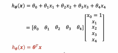
벡터로 표현하면 어차피 1차식이다.
4. 집값 예측
fetch_california_housing으로 진행했다.
from sklearn.datasets import fetch_california_housing
housing = fetch_california_housing()

df = pd.DataFrame(housing.data, columns=housing.feature_names)
df['Price'] = housing.target
import plotly.express as px
fig = px.histogram(df, x='Price')
fig.show()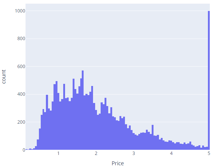
corr_mat = df.corr().round(1)
sns.heatmap(data=corr_mat, annot=True, cmap='bwr')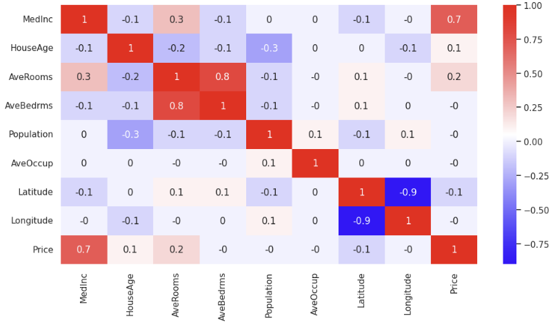
sns.set_style('darkgrid')
sns.set(rc={'figure.figsize': (12, 6)})
sns.regplot(x='MedInc', y='Price', data=df)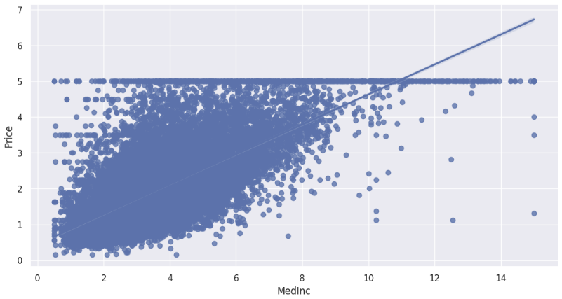
from sklearn.model_selection import train_test_split

X = df.drop(['Price'], axis=1)
y = df['Price']
X_train, X_test, y_train, y_test = train_test_split(X, y, test_size=0.2, random_state=13)
from sklearn.linear_model import LinearRegression
reg = LinearRegression()
reg.fit(X_train, y_train)LinearRegression도 OLS를 사용하고 있다.
from sklearn.metrics import mean_squared_error

pred_tr = reg.predict(X_train)
pred_test = reg.predict(X_test)
rmse_tr = np.sqrt(mean_squared_error(y_train, pred_tr))
rmse_test = np.sqrt(mean_squared_error(y_test, pred_test))

rmse_tr, rmse_test

>>>
(10.197682788069542, 9.302204905816124)
# 성능 확인
plt.scatter(y_test, pred_test)
plt.xlabel('Real Prices')
plt.ylabel('Predicted Prices')
plt.title('Real vs Predicted')
plt.plot([0, 6], [0, 6], 'r') # (0, 0) ~ (6, 6)
plt.show()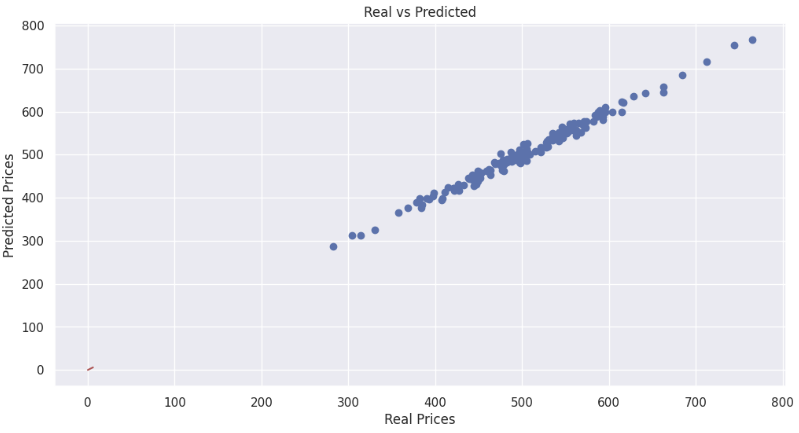
✨특성을 이해하려고 노력하자!
예측하는데 있어서 필요한 특성인가?
어떤 특성을 제외하고 RMSE를 확인했을 때 RMSE가 올라갔다고 해서(성능이 나빠짐) 그 특성을 무조건 제외해야 하는 건 아니다.