
문제 정의
예약 취소와 노쇼로 인해서 영업 이익이 감소하고 있다.
그래서 호텔 예약 취소와 노쇼 비율 현황 파악 및 고객 특성별 데이터를 확인 및 분석.
데이터 확인
데이터 및 소스코드 : GitHub
- 데이터 상세
-
hotel is_canceled lead_time arrival_date_year arrival_date_month arrival_date_week_number 호텔명 취소여부 입실까지 남은일 년 월 일 -
arrival_date_day_of_month stays_in_weekend_nights stays_in_week_nights adults children babies 일 주말여부 평일여부 성인 어린이 영유아 -
meal country market_segment distribution_channel is_repeated_guest previous_cancellations 식사 나라 예약유통채널상세 예약유통채널 기존고객여부 과거 취소한 예약수 -
previous_bookings_not_canceled reserved_room_type assigned_room_type booking_changes deposit_type agent 과거 취소하지않은 예약수 예약객실타입 배정된객실타입 예약변경횟수 보증금여부 여행사ID -
company days_in_waiting_list customer_type adr required_car_parking_spaces total_of_special_requests 예약지불회사 대기자 명단에 있었던 일수 계약타입 평균객실비용 요구주차대수 특별요청수 -
reservation_status reservation_status_date 예약상태 예약상태 업데이트 날짜
데이터 EDA & 전처리
기본 데이터 확인
데이터의 특성도 많고 샘플 데이터도 많다.
df.shape
>
(119390, 32)
데이터의 기본 정보를 보았을 때 결측치가 있음이 파악이 된다.
df.info()
>
<class 'pandas.core.frame.DataFrame'>
RangeIndex: 119390 entries, 0 to 119389
Data columns (total 32 columns):
 #   Column                          Non-Null Count   Dtype
---  ------                          --------------   -----
 0   hotel                           119390 non-null  object
 1   is_canceled                     119390 non-null  int64
 2   lead_time                       119390 non-null  int64
 3   arrival_date_year               119390 non-null  int64
 4   arrival_date_month              119390 non-null  object
 5   arrival_date_week_number        119390 non-null  int64
 6   arrival_date_day_of_month       119390 non-null  int64
 7   stays_in_weekend_nights         119390 non-null  int64
 8   stays_in_week_nights            119390 non-null  int64
 9   adults                          119390 non-null  int64
 10  children                        119386 non-null  float64
 11  babies                          119390 non-null  int64
 12  meal                            119390 non-null  object
 13  country                         118902 non-null  object
 14  market_segment                  119390 non-null  object
 15  distribution_channel            119390 non-null  object
 16  is_repeated_guest               119390 non-null  int64
 17  previous_cancellations          119390 non-null  int64
 18  previous_bookings_not_canceled  119390 non-null  int64
 19  reserved_room_type              119390 non-null  object
 20  assigned_room_type              119390 non-null  object
 21  booking_changes                 119390 non-null  int64
 22  deposit_type                    119390 non-null  object
 23  agent                           103050 non-null  float64
 24  company                         6797 non-null    float64
 25  days_in_waiting_list            119390 non-null  int64
 26  customer_type                   119390 non-null  object
 27  adr                             119390 non-null  float64
 28  required_car_parking_spaces     119390 non-null  int64
 29  total_of_special_requests       119390 non-null  int64
 30  reservation_status              119390 non-null  object
 31  reservation_status_date         119390 non-null  object
dtypes: float64(4), int64(16), object(12)
결측치
4개의 특성에서 결측치가 존재한다.
df.isnull().sum()
>
hotel                                  0
is_canceled                            0
lead_time                              0
arrival_date_year                      0
arrival_date_month                     0
arrival_date_week_number               0
arrival_date_day_of_month              0
stays_in_weekend_nights                0
stays_in_week_nights                   0
adults                                 0
children                               4 <<
babies                                 0
meal                                   0
country                              488 <<
market_segment                         0
distribution_channel                   0
is_repeated_guest                      0
previous_cancellations                 0
previous_bookings_not_canceled         0
reserved_room_type                     0
assigned_room_type                     0
booking_changes                        0
deposit_type                           0
agent                              16340 <<
company                           112593 <<
days_in_waiting_list                   0
customer_type                          0
adr                                    0
required_car_parking_spaces            0
total_of_special_requests              0
reservation_status                     0
reservation_status_date                0
dtype: int64
children 특성은 최빈값으로으로 치환할 것이다.
총 5개의 특성이 나타나고 있으며 가장 많은 대표값은 0이기에, 0으로 변환한다.
print(df['children'].nunique())
print(df['children'].unique())
>
5
[ 0.  1.  2. 10.  3. nan]

df.groupby('children', as_index=False)['agent'].count().sort_values(by='agent', ascending=False)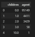
country은 다양하게 나타나고 있으며, 0값에도 일정한 나라가 지정되어 있기에 문자형으로 'none'로 표기하도록 한다.
print(df['country'].nunique())
print(df['country'].unique())
>
177
['PRT' 'GBR' 'USA' 'ESP' 'IRL' 'FRA' nan 'ROU' 'NOR' 'OMN' 'ARG' 'POL'
 'DEU' 'BEL' 'CHE' 'CN' 'GRC' 'ITA' 'NLD' 'DNK' 'RUS' 'SWE' 'AUS' 'EST'
 'CZE' 'BRA' 'FIN' 'MOZ' 'BWA' 'LUX' 'SVN' 'ALB' 'IND' 'CHN' 'MEX' 'MAR'
 'UKR' 'SMR' 'LVA' 'PRI' 'SRB' 'CHL' 'AUT' 'BLR' 'LTU' 'TUR' 'ZAF' 'AGO'
 'ISR' 'CYM' 'ZMB' 'CPV' 'ZWE' 'DZA' 'KOR' 'CRI' 'HUN' 'ARE' 'TUN' 'JAM'
 'HRV' 'HKG' 'IRN' 'GEO' 'AND' 'GIB' 'URY' 'JEY' 'CAF' 'CYP' 'COL' 'GGY'
 'KWT' 'NGA' 'MDV' 'VEN' 'SVK' 'FJI' 'KAZ' 'PAK' 'IDN' 'LBN' 'PHL' 'SEN'
 'SYC' 'AZE' 'BHR' 'NZL' 'THA' 'DOM' 'MKD' 'MYS' 'ARM' 'JPN' 'LKA' 'CUB'
 'CMR' 'BIH' 'MUS' 'COM' 'SUR' 'UGA' 'BGR' 'CIV' 'JOR' 'SYR' 'SGP' 'BDI'
 'SAU' 'VNM' 'PLW' 'QAT' 'EGY' 'PER' 'MLT' 'MWI' 'ECU' 'MDG' 'ISL' 'UZB'
 'NPL' 'BHS' 'MAC' 'TGO' 'TWN' 'DJI' 'STP' 'KNA' 'ETH' 'IRQ' 'HND' 'RWA'
 'KHM' 'MCO' 'BGD' 'IMN' 'TJK' 'NIC' 'BEN' 'VGB' 'TZA' 'GAB' 'GHA' 'TMP'
 'GLP' 'KEN' 'LIE' 'GNB' 'MNE' 'UMI' 'MYT' 'FRO' 'MMR' 'PAN' 'BFA' 'LBY'
 'MLI' 'NAM' 'BOL' 'PRY' 'BRB' 'ABW' 'AIA' 'SLV' 'DMA' 'PYF' 'GUY' 'LCA'
 'ATA' 'GTM' 'ASM' 'MRT' 'NCL' 'KIR' 'SDN' 'ATF' 'SLE' 'LAO']

 # 데이터 상세 확인
 df.groupby(['country'], as_index=False)['agent'].count().sort_values(by='agent', ascending=False)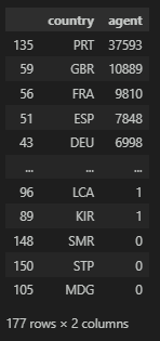
agent와 company은 여행사나 호텔 관련 사업체를 통하지 않고 개인적으로 예약을 할 수도 있는 부분이다. 특히 company의 결측치 값이 매우 많은 것으로 보아, 특정 사업체를 거치지 않고 개인 예약이 많다는 것을 확인할 수 있다.
그래서 결측치 값은 아이디가 부여되지 않는 0값으로 대체한다.
# 결측치 대체
df['children'].fillna(0, inplace=True)
df['country'].fillna('none', inplace=True)
df['agent'].fillna(0, inplace=True)
df['company'].fillna(0, inplace=True)

df.isnull().sum().sum()
>
0
이상치
adr(평균객실비용)에서 음수의 값이 존재한다.
취소나 노쇼 등으로 인한 객실 비용이지 아니면 다른 사유에서 음수의 값이 있는지 모른다. 데이터를 분석에 있어 불필요한 요소라 판단하고 삭제하기로 한다. 더욱이 세부 사항을 보면 음수 값은 1개의 샘플만 가지므로 삭제해도 무방할 것으로 보인다.
(df.describe() < 0).sum()
>
is_canceled                       0
lead_time                         0
arrival_date_year                 0
arrival_date_week_number          0
arrival_date_day_of_month         0
stays_in_weekend_nights           0
stays_in_week_nights              0
adults                            0
children                          0
babies                            0
is_repeated_guest                 0
previous_cancellations            0
previous_bookings_not_canceled    0
booking_changes                   0
agent                             0
company                           0
days_in_waiting_list              0
adr                               1
required_car_parking_spaces       0
total_of_special_requests         0
dtype: int64

# 음수 데이터 샘플 개수
len(df[df['adr'] < 0])
>
1

# 데이터 삭제(음수가 아닌 데이터만 재정의)
df = df[df['adr'] >= 0]
클레스 불균형
이러한 데이터들이 늘 그러한 경향을 보이듯, 클래스 불규형이 심각한 수준이다.
df['reservation_status'].value_counts()
>
Check-Out    75166
Canceled     43017
No-Show       1207
Name: reservation_status, dtype: int64
각 label data별 비율 - 63%(정상) : 36%(취소) : 1%(노쇼)
# 정상
df['reservation_status'].value_counts()[0] / df['reservation_status'].value_counts().sum()
>
62.958371722924866

# 취소
df['reservation_status'].value_counts()[1] / df['reservation_status'].value_counts().sum() * 100
>
36.03065583382193

# 노쇼
df['reservation_status'].value_counts()[2] / df['reservation_status'].value_counts().sum() * 100
>
1.010972443253204
이상치를 지금 판별하기에는 용이하지 않으니 탐색을 하면서 살펴본다.
일자별 탐색
# 년
df['arrival_date_year'].value_counts()
>
2016 56707
2017 40687
2015 21996
Name: arrival_date_year, dtype: int64
# 월
df['arrival_date_month'].value_counts()
>
August 13877
July 12661
May 11791
October 11160
April 11089
June 10939
September 10508
March 9794
February 8068
November 6794
December 6780
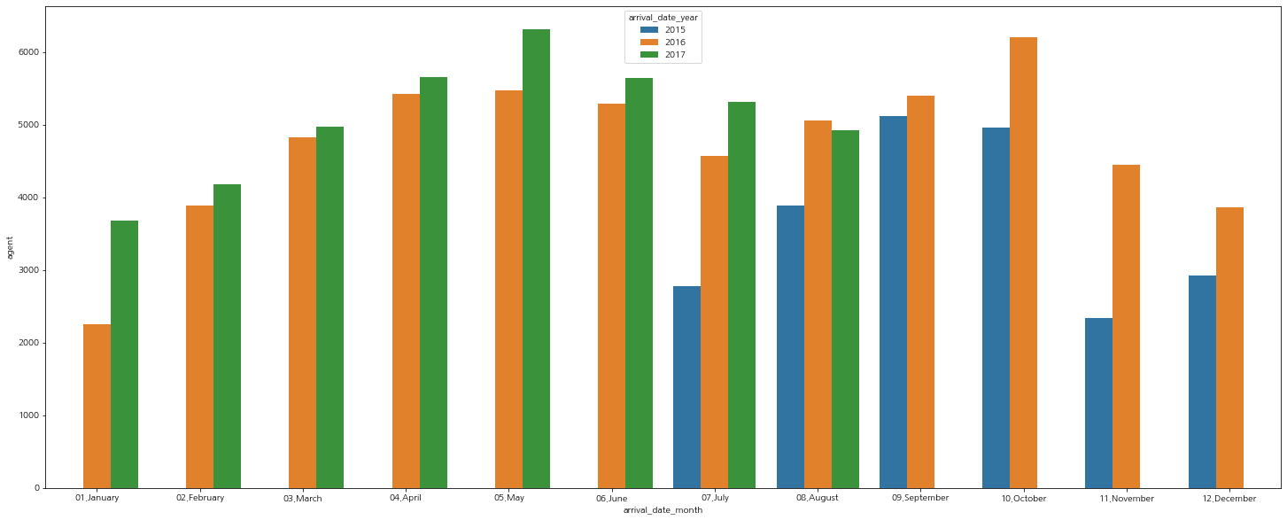
January 5929년/월로 묶어서 살펴본다.
df.groupby(['arrival_date_year', 'arrival_date_month'], as_index=False)['agent'].count()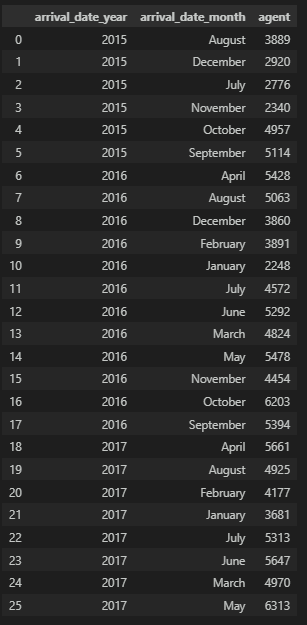
해당 년의 월을 정렬하기 위해 컬럼을 재정의하고 다시 보자.
# 월 재정의(숫자로 정렬하기 위해)
to_dicts = {'January' : '01.January',
            'February' : '02.February',
            'March' : '03.March',
            'April' : '04.April',
            'May' : '05.May',
            'June' : '06.June',
            'July' : '07.July',
            'August' : '08.August',
            'September' : '09.September',
            'October' : '10.October',
            'November' : '11.November',
            'December' : '12.December'}

# 년-월 그룹핑
df_res = df.groupby(['arrival_date_year', 'arrival_date_month'], as_index=False)['agent'].count()

# 컬럼 내용 변경
df_res = df_res.replace(to_dicts)

# 정렬
df_res.sort_values(by=['arrival_date_year', 'arrival_date_month'])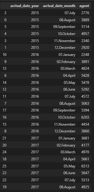
이렇게 정렬하면 그래프로 그려 볼 때에도 용이해진다.
클래스 별 탐색
취소와 노쇼는 손실 비용으로 같은 카테고리로 묶어서 구분하기로 한다.
# 취소와 노쇼에 대한 데이터 1로 변경
import numpy as np
df['reservation_status'] = np.where(df['reservation_status'] != 'Check-Out', 1, 0)
df['reservation_status'].value_counts()
# 비율 : 37%로 취소 또는 노쇼 고객 비율
df['reservation_status'].value_counts()[1] / df['reservation_status'].value_counts().sum() * 100
>
37.04193853705115월 별
catplot 그래프로 월별 추이를 확인해 보자.
특별한 인사이트는 보이지 않는다.
sns.catplot(x="arrival_date_month", hue="reservation_status", kind="count",palette="pastel", edgecolor=".6",data=df, aspect=3,
            order = ['January', 'February', 'March', 'April', 'May', 'June', 'July', 'August', 'September', 'October', 'November', 'December'])
plt.gcf().set_size_inches(20, 8)
plt.show()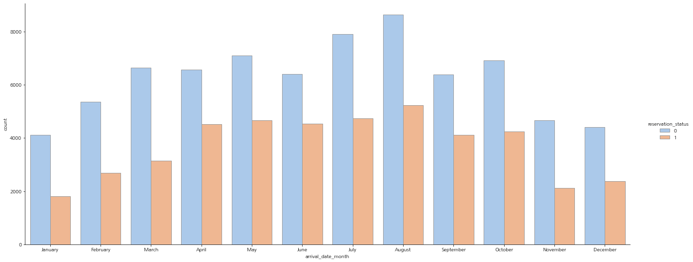
추가적으로 월별 취소/노쇼 비율을 확인해보자.
4, 5, 6월이 다른 달에 비해서 취소 및 노쇼 비율이 높다.
# 월에 따른 취소/노쇼율 비교
df_gp = df.groupby('arrival_date_month')['reservation_status'].agg(['count','sum']).reset_index()
df_gp['ratio'] = round((df_gp['sum'] / df_gp['count']) * 100, 1)
df_gp['arrival_date_month'].replace(to_dicts, inplace=True)
df_gp = df_gp.sort_values(by=['ratio'], ascending=False)
df_gp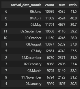
호텔 별
호텔의 종류가 2가지로 나뉜다.
City Hotel의 노쇼 비율이 더 높은 것이 확인 된다.
df['hotel'].value_counts()
>
City Hotel      79330
Resort Hotel    40059
Name: hotel, dtype: int64

# catplot으로 Resort Hottel과 City Hotel 비교
sns.catplot(x="hotel", hue="reservation_status", kind="count",palette="pastel", edgecolor=".6",data=df, aspect=3)
plt.gcf().set_size_inches(20, 8)
plt.show()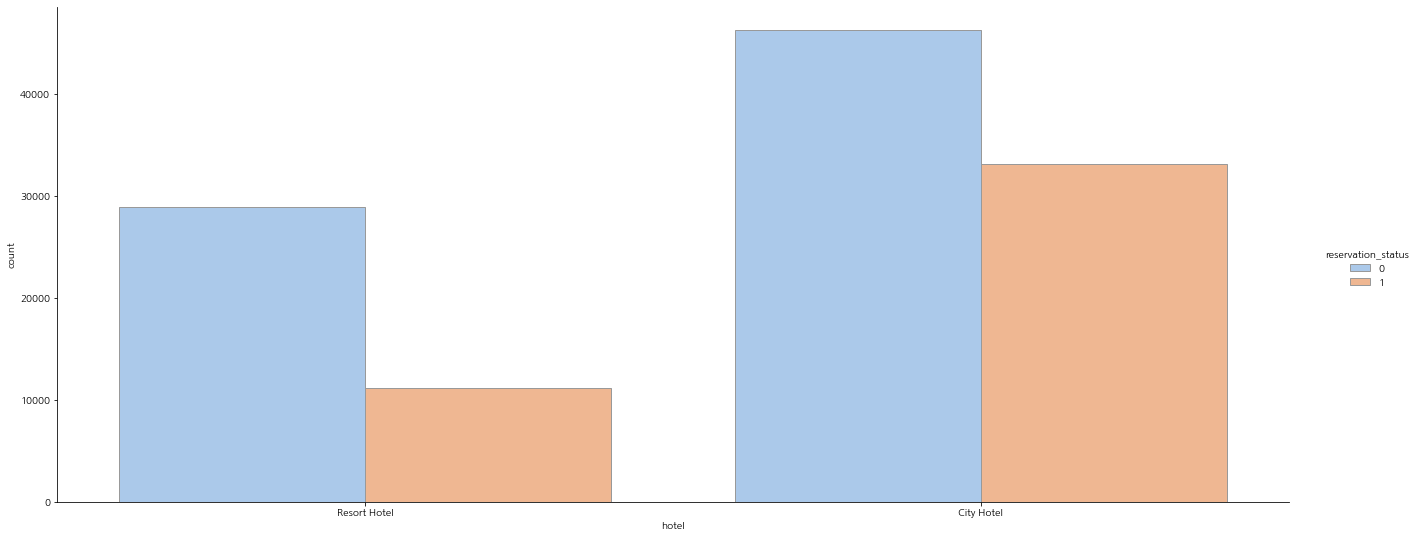
호텔 별로 상세 비율을 확인해보자.
예약 건수도 City Hotel이 더 높고, 비율도 City Hotel이 더 높은 것을 보아서 예약 당시의 환불 정책이나 다른 사항들을 살펴볼 필요성이 있다.
또한 Resort Hotel과 City Hotel의 비율의 차이가 심해서, 모델링을 한다면 따로 분리하는 것도 염두에 두자.
# Resort Hotle과 City Hotel 비교
df_gp = df.groupby('hotel')['reservation_status'].agg(['count','sum'])
df_gp['ratio'] = round((df_gp['sum'] / df_gp['count']) * 100, 1)
df_gp = df_gp.sort_values(by=['ratio'], ascending=False)
df_gp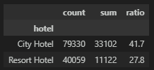
주말 예약 일수
주말을 끼고 예약을 하는 비율은 43.5%로 높은 비율을 나타낸다.
df['stays_in_weekend_nights'].value_counts()[0] / df['stays_in_weekend_nights'].value_counts().sum() * 100
>
43.553426195043095
주말을 포함시키는 예약의 일수를 그래프로 확인해보자.
0은 평일이므로 제외시키면, 토요일과 일요일을 포함하게 되면 1아니면 2가 가장 많다. 그리고 7일 이상을 머무르게 되면 주말이 포함이 더 될 것인데 아무래도 장기 투숙 비율은 적을 것이란 예상과 일치한다.
# 주말 예약 일수에 따른 비교
sns.catplot(x="stays_in_weekend_nights", hue="reservation_status", kind="count", palette="pastel", edgecolor=".6", data=df, aspect=3)
plt.gcf().set_size_inches(20, 8)
plt.show()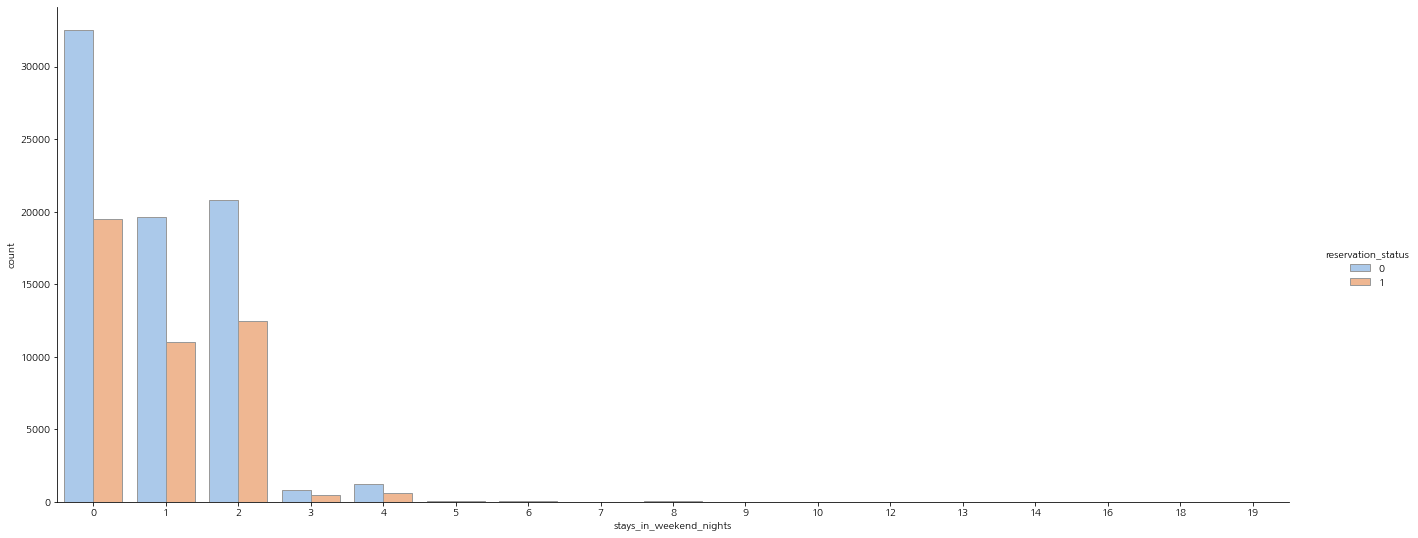
좀 더 자세히게 주말 예약 일수에 따른 비교를 확인해보면, 일수가 3일이 넘어가는 일수들은 건수가 너무 낮아서 유의미하게 구별이 되지 않을 것 같다.
# 주말 예약 일수에 따른 비교
df_gp = df.groupby('stays_in_weekend_nights')['reservation_status'].agg(['count','sum'])
df_gp['ratio'] = round((df_gp['sum'] / df_gp['count']) * 100, 1)
df_gp = df_gp.sort_values(by=['ratio'], ascending=False)
df_gp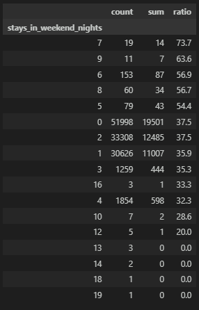
그룹을 묶어서, 주말을 포함하지 않으면 0, 주말을 2일 이하로 포함하면 1을, 3일 이상은 2로 하고 확인해보자.
유의미한 변수로 작용할 것 같아 보이지는 않는다.
# ▶ 주말 예약 일수에 따른 비교(re-binning)
df_c = df.copy()

df_c['gp'] = np.where(df_c['stays_in_weekend_nights'] <= 2, 1, np.where(df_c['stays_in_weekend_nights'] <= 8, 2, 3))

df_gp = df_c.groupby('gp')['reservation_status'].agg(['count','sum'])
df_gp['ratio'] = round((df_gp['sum'] / df_gp['count']) * 100, 1)
df_gp = df_gp.sort_values(by=['ratio'], ascending=False)
df_gp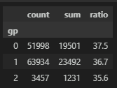
객실 타입 별
객실의 타입별로 확인해보자.
A 타입의 건수가 가장 많고 그 다음으로 D 타입이다. 나머지는 유의미한 변수로 보기엔 어려울 수도 있을 것 같다.
sns.catplot(x="reserved_room_type", hue="reservation_status", kind="count",palette="pastel", edgecolor=".6",data=df, aspect=3)
plt.gcf().set_size_inches(20, 8)
plt.show()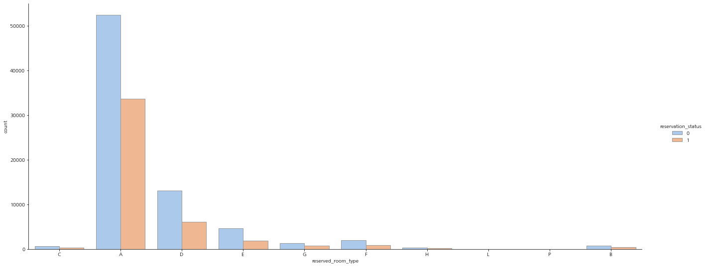
클래스 비율을 보면 P 타입은 100%로 취소/노쇼다. 하지만 건수가 적어서 유의미하게 보기엔 어렵다.
다음으로 건수가 가장 많은 A 타입의 경우 취소/노쇼의 비율이 높아서 신경써야 하는 부분으로 이슈로 다뤄봐야 할 것 같아 보인다.
df_gp = df.groupby('reserved_room_type')['reservation_status'].agg(['count','sum'])
df_gp['ratio'] = round((df_gp['sum'] / df_gp['count']) * 100, 1)
df_gp = df_gp.sort_values(by=['ratio'], ascending=False)
df_gp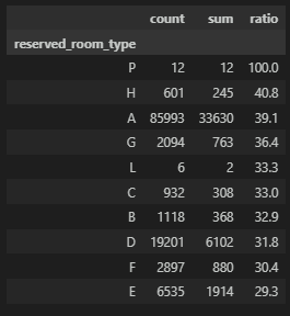
lead time
예약일까지 남아있는 일수로 살펴보면, 예약일이 가까워졌을 때 취소가 될 확률이 높을 것으로 예상이 된다. 분포를 확인해보면 예약일로부터 가까울수록 건수가 많다.
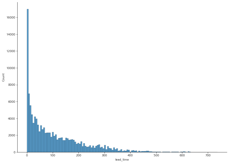
그렇다면 lead time별로 구간화를 하여 취소 여부를 확인해보자.
1부터 시작하여 일수가 커질수록 수를 키워가며 5구간으로 확인해보자.
예상했던 것과는 반대로 거리가 가까울수록 취소를 하는 확률이 낮아지며, 오히려 예약 날짜가 많을 남았을 때 취소 비율이 더 높다. 이것은 예약할 때의 예약 비용이나 환불 정책을 참고하면 더 좋을 것 같다.
# lead time 구간화
df_c = df.copy()
df_c['gp'] = np.where(df['lead_time'] <= 10, 1, np.where(df['lead_time']<=50, 2, np.where(df['lead_time']<=100, 3, np.where(df['lead_time']<=200, 4, np.where(df['lead_time']<=300, 2, 5)))))

df_gp = df_c.groupby('gp')['reservation_status'].agg(['count','sum'])
df_gp['ratio'] = round((df_gp['sum'] / df_gp['count']) * 100, 1)
df_gp = df_gp.sort_values(by=['ratio'], ascending=False)
df_gp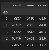
수치형 변환
모델링을 위해 문자형 데이터를 수치화한다.
# category feature 확인
num_list = []
cate_list = []

for col in df.columns:
    if df[col].dtypes == 'O':
        cate_list.append(col)
    else:
        num_list.append(col)

# LabelEncoder()을 사용하여 수치형으로 변환
for col in cate_list:
    le = LE()
    le.fit(df[col])
    df[col] = le.transform(df[col])
모델링
트리 계열의 앙상블과 부스팅 방법인 RandomForestClassifier와 LGBMClassifier를 사용하도록 한다.
그리고 평가지표는 f1 score를 사용한다.
데이터 나누기
학습/평가 데이터와 label데이터 분리
# Label data 분리
X = df.drop(['is_canceled', 'reservation_status_date', 'reservation_status'], axis=1)
Y = df['reservation_status']

# 학습/평가 데이터 분리
train_x, test_x, train_y, test_y = train_test_split(X, Y, stratify=Y)

train_x.shape, train_y.shape, test_x.shape, test_y.shape
>
((89541, 29), (89541,), (29848, 29), (29848,))
하이퍼 파라미터 튜닝
model_param_dict = {}
rfc_param_grid = ParameterGrid({
                                'max_depth':[3, 10, 15, 30, 50],
                                'n_estimators':[200, 400, 800],
                                'random_state':[29, 1000],
                                'n_jobs':[-1]
})
lgbm_param_grid = ParameterGrid({
                                'max_depth':[3, 10, 15, 30, 50],
                                'n_estimators':[200, 400, 800],
                                'learning_rate':[0.05, 0.1, 0.2]
})

model_param_dict[RFC] = rfc_param_grid
model_param_dict[LGBM] = lgbm_param_grid
학습
best_score = -1
num_iter = 0

for m in model_param_dict.keys():
    for p in model_param_dict[m]:
        model = m(**p).fit(train_x.values, train_y.values)
        pred = model.predict(test_x.values)
        score = metrics.f1_score(test_y.values, pred)

        if best_score < score:
            best_score = score
            best_model = m
            best_param = p

        num_iter += 1

        print(f'iteration {num_iter}/{max_iter} - best score : {best_score}')
최종 모델 선정 및 평가지표 확인
모델 선정
model = best_model(**best_param)
model.fit(train_x.values, train_y.values)
classification_report 확인
train_pred = model.predict(train_x)
tet_pred = model.predict(test_x)
print(metrics.classification_report(train_y, train_pred))
print(metrics.classification_report(test_y, tet_pred))
>
precision recall f1-score support
0 0.99 1.00 1.00 56373
1 0.99 0.99 0.99 33168
accuracy 0.99 89541
macro avg 0.99 0.99 0.99 89541
weighted avg 0.99 0.99 0.99 89541
precision recall f1-score support
0 0.90 0.94 0.92 18792
1 0.88 0.82 0.85 11056
accuracy 0.90 29848
macro avg 0.89 0.88 0.89 29848
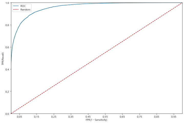
weighted avg 0.89 0.90 0.89 29848roc_auc score 확인
train_proba = model.predict_proba(train_x)[:, 1]
test_proba = model.predict_proba(test_x)[:, 1]

train_score = metrics.roc_auc_score(train_y, train_proba)
test_score = metrics.roc_auc_score(test_y, test_proba)

print('train roc_auc score :', train_score)
print('test roc_auc score : ', test_score)
>
train roc_auc score : 0.999534536332405
test roc_auc score :  0.9605016672927607
test에 대한 roc_auc score를 그래프로 확인해보자.
중요 변수 파악
features_importance = model.feature_importances_
features_importance = pd.Series(features_importance, index=train_x.columns)
features_top = features_importance.sort_values(ascending=False)

plt.figure(figsize=(16, 12))
plt.title('Feature Importance')
sns.barplot(x=features_top, y=features_top.index)
plt.show()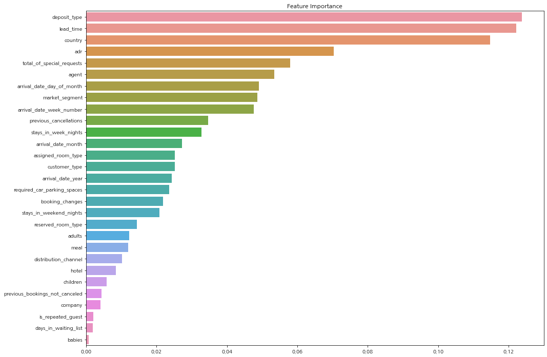
중요 변수 상세
상세히 보지 않았던 특징들 중에서 중요 변수라 파악된 변수들을 다시 살펴보자.
데이터를 수치로 바꿨기에 다시 raw data를 불러와서 확인해본다.
보증금(deposit type)
보증금 형태 중에서 환불이 되지 않는 보증금의 경우에 취소 비율이 매우 높다.
sns.catplot(x='deposit_type', hue='reservation_status', kind='count', palette='pastel', edgecolor='.6', data=data, aspect=3)
plt.gcf().set_size_inches(25, 8)
plt.show()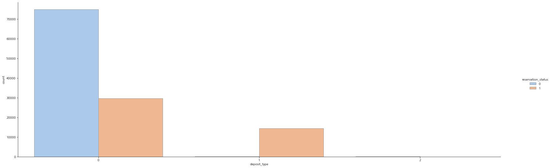
# 월에 따른 취소/노쇼율 비교 - 환불 불가인데, 취소율이 높다
df_gp = data.groupby('deposit_type')['reservation_status'].agg(['count','sum'])
df_gp['ratio'] = round((df_gp['sum'] / df_gp['count']) * 100, 1)
df_gp = df_gp.sort_values(by=['ratio'], ascending=False)
df_gp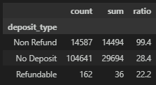
Country
나라에 따라서도 취소율은 유의미하게 나타난다. 특히 PRT(포르투칼)은 취소율이 높아서 고위험군으로 보고 관리해야 하는 부분이 있다.
# Country
df_gp = data.groupby('country')['reservation_status'].agg(['count','sum'])
df_gp['ratio'] = round((df_gp['sum'] / df_gp['count']) * 100, 1)
df_gp = df_gp.sort_values(by=['ratio'], ascending=False)
df_gp[df_gp['count'] > 2000]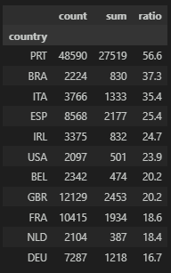
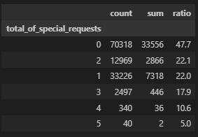
total of special requests
호텔에 머물 의향이 높을 수록 요청사항도 높을 것이라 판단이 되는 부분이다.
기대 효과
예약 취소 및 노쇼 고객 손실 비용 절감 및 파악을 하여 영업 이익의 증대와 수요를 파악(ex. 취소/노쇼 가능성이 높은 객실에 대하여 다른 예약으로 대체)하여 호텔 운영에 도움