데이터 출처 및 문제
1. 출처
서울/부산 지역 아파트 실 거래가를 예측하는 모델 개발 경진 대회
- 제공 : DACON - 직방
- data download : DACON-아파트 실거래가 예측
- 소스 코드(& smaple data) : GitHub
데이터
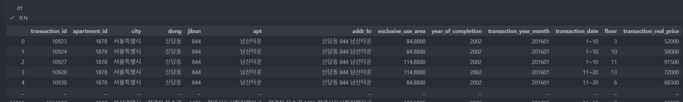
train.csv : 모델 학습용 데이터
- transaction_real_price : 실거래가(라벨 : train.csv에만 존재)
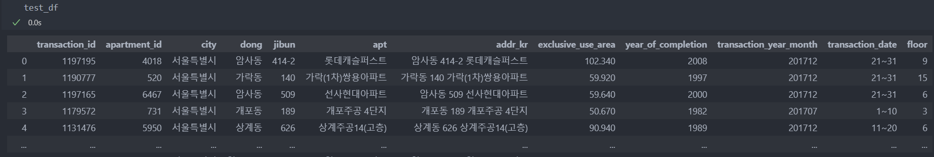
test.csv : 모델 평가용 데이터
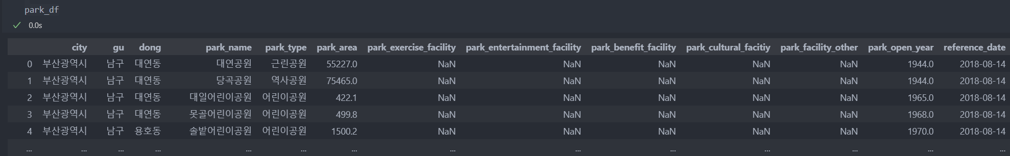
park.csv : 서울/부산 지역의 공원에 대한 정보
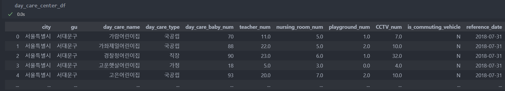
day_care_center.csv : 서울/부산 지역의 어린이집에 대한 정보
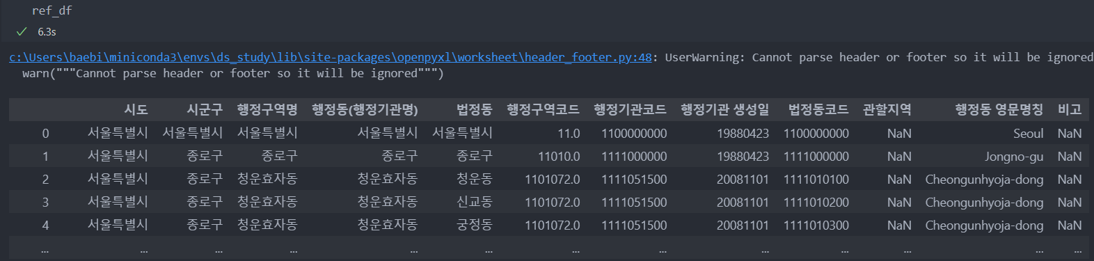
한국행정구역분류.xlsx(참조 데이터: 외부자료) : '구' 정보를 위해
-
train.csv
-
test.csv
-
park.csv
-
day_care_center.csv
-
한국행정구역분류.xlsx
데이터 탐색 및 전처리
1. 변수 추가
train 데이터에는 '구' 정보가 없고, 어린이집 데이터에는 '동' 정보가 없어 병합할 때 문제가 될 수 있으다.
외부 참조 데이터 행정구역분류 데이터를 바탕으로 '구'변수를 추가하도록 한다.
참조 데이터의 '시도'컬럼
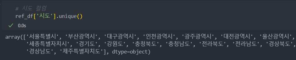
# 서울과 부산 '시도' 컬럼만
ref_df = ref_df.loc[ref_df['시도'].isin(['서울특별시', '부산광역시'])]
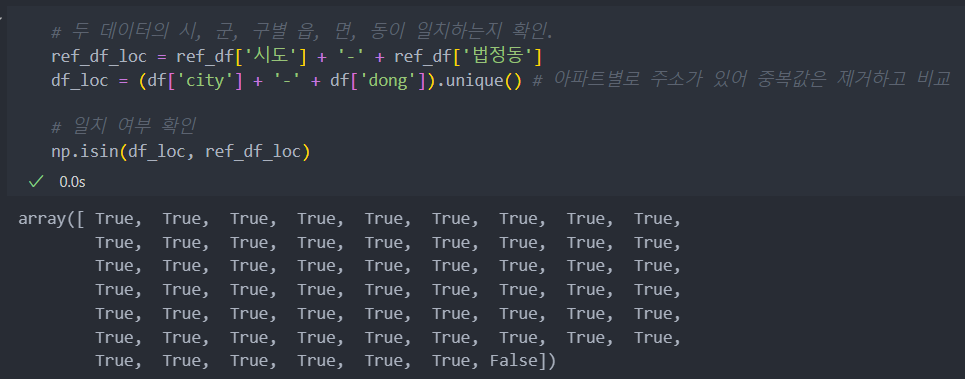
ref_df = ref_df[['시도', '시군구', '법정동']]주소 데이터를 다룰 때에 신경써야 할 부분이 있다.
'구'컬럼을 병합하기 전에, '행정동' 혹은 '법정동' 기준으로 주소가 입력되어 있을 수 있다.(보통은 '법정동' 기준으로 주소 기제)
그래서 병합하려는 두 데이터의 시, 군, 구, 동 등 일치하지 않는 경우가 있을 수 있어 확인해야 한다.
그리고 '구'의 이름이 '중구' 등 같은 이름이 있을 수 있으니 데이터를 합치거나 분리 및 평균 등의 작업을 할 때에는 '계층화'를 해서 전처리를 해야한다.
일치하지 않는 주소가 있다는 것을 확인하였다.
train 데이터에는 읍/리 까지 주소가 기제되어 있고 행정구역 데이터에는 읍만 기제되어 있어 '리'부분을 삭제해야 merge 할 때 일치하여 문제가 없다.
# 읍과 리가 있는 경우 '리' 부분 제거
df['dong'] = df['dong'].str.split(' ', expand=True).iloc[:, 0]
행정구역 데이터는 '행정동'별로도 주소가 기제되어 있어서 '법정동'의 데이터에 중복이 있을 수 있어서 중복되어 있다면 삭제한다.
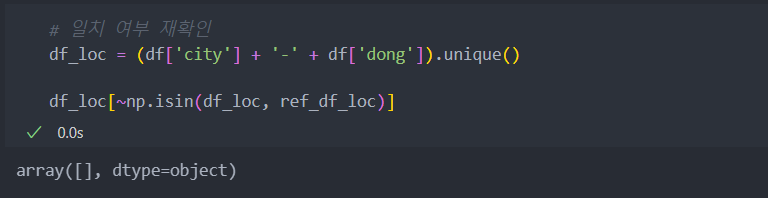
# 시도와 법정동이 완전히 똑같은 행 제거
ref_df = ref_df.drop_duplicates(subset=['시도', '법정동'])
일치 여부 다시 확인 후 merge
# df, ref_df 병합하여 '구' 컬럼 추가
df = pd.merge(df, ref_df, left_on=['city', 'dong'], right_on=['시도', '법정동'])

# 합친 후 ref_df 부분에 있던 '시도', '법정동' 컬럼 삭제 후 '구'컬럼만 남겨두기
df.drop(['시도', '법정동'], axis=1, inplace=True)
2. 중복 및 불필요한 변수 제거
# 거래 id는 불필요하다 판단, addr은 중복으로 제거
df.drop(['transaction_id', 'addr_kr'], axis=1, inplace=True)
3. 변수 탐색
문자로 되어 있는 변수를 수치형으로 변환(서울 : 1, 부산: 0)
아파트가 지어진지 얼마나 되었는지, 거래 년도는 언제인지 확인하고 수치화.
아파트의 층수가 시세에 영향을 끼치는 층수 범위를 수치화.
서울지역과 부산지역을 범주형 변수 수치형으로 변환한 컬럼 추가
# 시 확인
df['city'].unique()
array(['서울특별시', '부산광역시'], dtype=object)

# 서울 : 1, 부산 : 0
df['seoul'] = (df['city'] == '서울특별시').astype(int)
아파트 나이 컬럼 추가.
# 아파트가 언제 건축되었는지 나이 변수로
df['age'] = 2018 - df['year_of_completion']
df.drop('year_of_completion', axis=1, inplace=True)
아파트 거래 년/월로 분리 컬럼 추가.
# 거래 년도
df['transaction_year_month'] = df['transaction_year_month'].astype(str) # 년/월 분리를 위해

df['transaction_year'] = df['transaction_year_month'].str[:4].astype(int)
df['transaction_month'] = df['transaction_year_month'].str[4:].astype(int)

df.drop('transaction_year_month', axis=1, inplace=True)
아파트의 층수가 시세에 영향을 미치는지 확인하고 층수를 그룹으로 묶어서 유의미하게 가격차가 발생하는 평균값을 보고 나눈다.
층별 시세를 막대 그래프로 확인.
보면 15, 25, 51, 72층을 기준으로 평균적인 가격이 조금 오르며 72층부터는 급격하게 오르는 모습을 보인다.
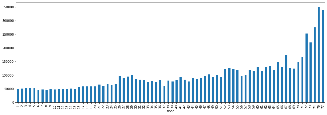
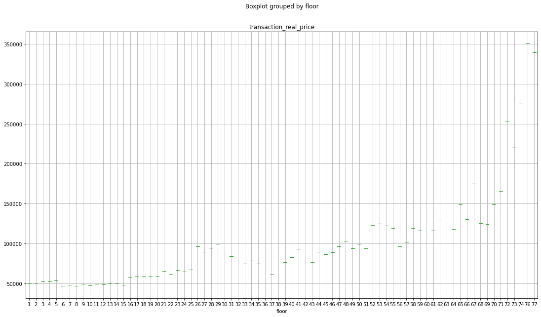
좀더 자세히 박스 플롯으로 층을 구분하여 평균가를 보자.
15층 이하
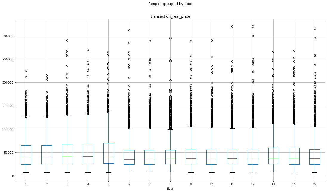
25층 이하
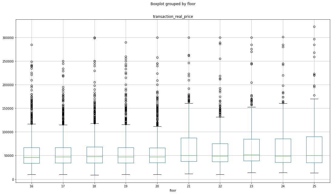
51층 이하
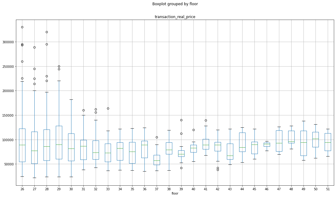
72층 이하
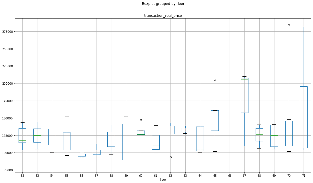
최상층
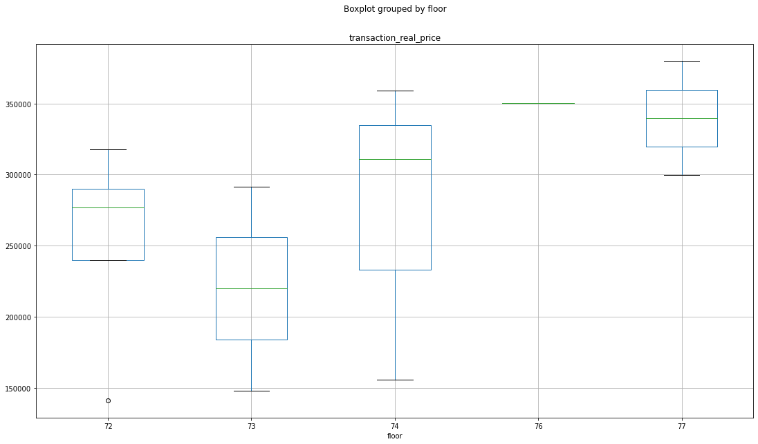
이렇게 5의 범주형 변수로 나누고 층 컬럼은 삭제하도록 한다.
4. 시세 변수 추가
시세는 해당 아파트가 위치하는 지리적 위치에 영향을 많이 받을 것이라 판단이 된다.
그리고 아파트 브렌드(시공사)에 따라서도 시세가 영향을 많이 받을 것이라 판단되기에 '구'별, 브렌드(아파트 id)별 평균 시세를 추가하기로 한다.
'구'는 시별로 이름이 같은, 예로 '중구'와 같이 '구' 이름이 같을 수 있으니 groupby를 할 때 '시'와 묶어서 계층화를 해주도록 한다.
# 구별 전체 평균 시세 추가
mean_price_per_gu = df.groupby(['city', '시군구'], as_index = False)['transaction_real_price'].mean()
mean_price_per_gu.rename({'transaction_real_price':'구별_전체_평균_시세'}, axis = 1, inplace = True)# axis=1 : 컬럼 이름/ axis=0 인덱스 이름 변경
df = pd.merge(df, mean_price_per_gu, on = ['city', '시군구'])

# 구별 작년 시세 추가
# price_per_gu_and_year 변수에 직접 수정을 하므로, df가 변경되는 것을 방지하기 위해, df.copy().groupby~를 사용
price_per_gu_and_year = df.copy().groupby(['city', '시군구', 'transaction_year'], as_index=False)['transaction_real_price'].agg(['mean', 'count']) # agg(): 2개 이상의 함수를 사용할 때 사용
price_per_gu_and_year = price_per_gu_and_year.reset_index().rename({'mean':'구별_작년_평균_시세', 'count':'구별_작년_거래량'}, axis=1)

price_per_gu_and_year['transaction_year'] += 1 # df 2018년 = price_per_gu_and_year 2017 + 1 이 되어 같은 년도로 merge를 하면 작년의 transaction_real_price가 추가된다.
df = pd.merge(df, price_per_gu_and_year, on=['city', '시군구', 'transaction_year'], how='left') # inner이 default로 교집합으로 합치면 작년 거래량이 없는 경우 빼고 병합된다. 이를 방지하기 위해 'left'를 기준으로 병합하고 작년 거래가 없으면 NaN값이 붙는다.
df['구별_작년_거래량'].fillna(0, inplace=True)

# 아파트(브랜드)별 평균 시세 추가
price_per_aid = df.copy().groupby(['apartment_id'], as_index=False)['transaction_real_price'].mean()
price_per_aid.rename({'transaction_real_price':'아파트별_평균가격'}, axis=1, inplace=True)

df = pd.merge(df, price_per_aid, on=['apartment_id'])
5. 공원 데이터 병합
아파트가 속한 지역 주변에 공원의 유무가 시세에 영향을 끼치는지(제공된 데이터이고 공원의 유무는 유의미한 변수가 될 것이라 판단(추가로 공원 외에도 편의시설 유무가 근처에 있는지 확인해 보는 것도 유의미할 것 같다))
공원의 'facility'들의 변수들이 너무 많아, 모든 값에 정의하는 것은 좋은 접근이 아닌 것 같으므로 시설이 있으면 1, 없으면 0으로 한다.
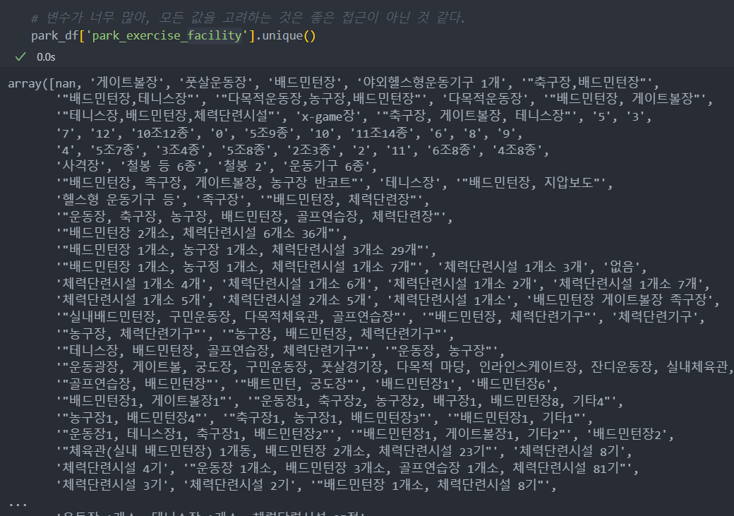
facility_cols = ['park_exercise_facility', 'park_entertainment_facility', 'park_benefit_facility', 'park_cultural_facitiy', 'park_facility_other']

# 범주 변수로 시설이 존재하면 1, 없으면 0으로
for col in facility_cols:
    park_df.loc[park_df[col].notnull(), col] = 1
    park_df.loc[park_df[col].isnull(), col] = 0
그리고 아파트 주변에 공원이 있다고 시세에 크게 영향을 줄 것 같지는 않다.
그래서 해당하는 동의 전체적인 편의시설인 공원의 수를 동의 복지개념으로 생각하여 '동'별 구분이 오히려 아파트 시세에 영향을 더 줄 것으로 판단되어, 동별 공원의 수와 동별 facility들의 수를 추가하도록 한다.
# 동별 공원 수
num_park_per_dong = park_df.groupby(['city', 'gu', 'dong'], as_index=False)['park_name'].count()
num_park_per_dong.rename({'park_name':'공원수'}, axis=1, inplace=True)

# 동별 공원에 배치된 facility 수
num_facility_per_dong = park_df.groupby(['city', 'gu', 'dong'], as_index=False)[facility_cols].sum()

# 공원수 데이터 추가
df = pd.merge(df, num_park_per_dong, left_on=['city', '시군구', 'dong'], right_on=['city', 'gu', 'dong'], how='left')
df['공원수'].fillna(0, inplace= True)
df.drop('gu', axis=1, inplace=True)

# 공원 facility 추가
df = pd.merge(df, num_facility_per_dong, left_on=['city', '시군구', 'dong'], right_on=['city', 'gu', 'dong'], how='left')
df[facility_cols].fillna(0, inplace=True)
df.drop('gu', axis=1, inplace=True)
6. 어린이집 데이터 병합
아파트가 속한 지역 주변에 어린이집 유무가 시세에 영향을 끼치는지(제공된 데이터이고 어린이집 유무는 유의미한 변수가 될 것이라 판단(추가로 초등/중등/고등학교 유무도 있으면 더 적절할 것 같다))
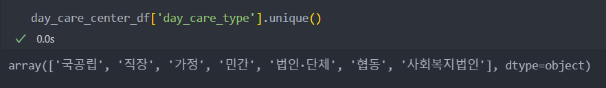
같은 어린이집이어도 종류가 다르면 아파트 가격에 다르게 영향을 줄 것이다.(개인가정, 사립, 공립)
그리고 아이가 있는 부모라면, 어린이집 수와 케어 가능한 아이의 수 등만 보고 아파트 구매를 결정할 것이다.
그래서 시/구별(동의 데이터가 없다) 어린이집 유형 및 케어 가능한 아이 수를 추가할 것이다.
# 필요한 컬럼만 쓰자.
day_care_center_df = day_care_center_df[['city', 'gu', 'day_care_type', 'day_care_baby_num']]

# 어린이집 종류를 더미화 하여 수치로 변환
dummy_day_care_type = pd.get_dummies(day_care_center_df['day_care_type'], drop_first=False)
dummy_day_care_type = dummy_day_care_type.add_prefix('어린이집유형_') # 어린이집유형_ + 컬럼명

day_care_center_df = pd.concat([day_care_center_df, dummy_day_care_type], axis=1) # axis=0은 행방향
day_care_center_df.drop('day_care_type', axis=1, inplace=True)

# 시/구별 모든 컬럼의 데이터 집계 :
aggregated_day_care_center_df = day_care_center_df.groupby(['city', 'gu'], as_index=False)[day_care_center_df.columns[2:]].sum()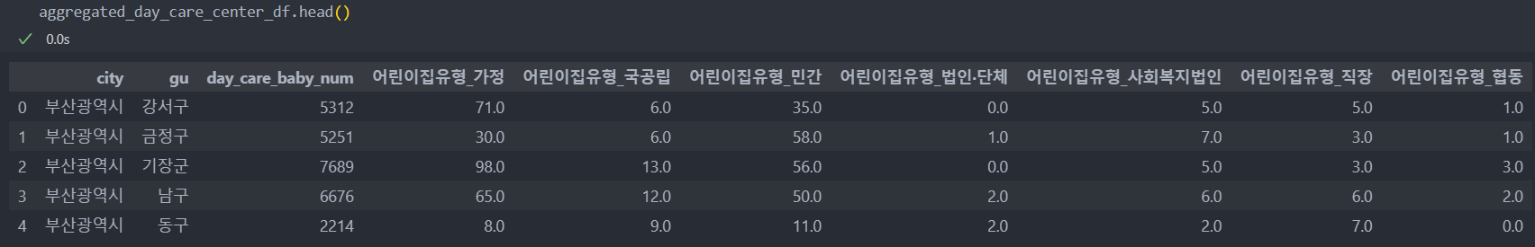
어린이집 데이터를 학습 데이터에 추가하도록 한다.
# 어린이집 데이터 추가
df = pd.merge(df, aggregated_day_care_center_df, left_on=['city', '시군구'], right_on=['city', 'gu'], how='left')
df[aggregated_day_care_center_df.columns].fillna(0, inplace=True)
df.drop('gu', axis=1, inplace=True)
모델링
참조 : 특징 선택
사용할 모델 : 데이터 샘플들이 많고 범주형과 연속형이 섞여있는 특징들이기에 트리 기반의 앙상블 모델들을 사용한다.
- RandomForestRegressor
- XGBRegressor
- LGBMRegressor
특징 선택
- 특징 선택 : 5, 10, 15, 20개 선택
- 통계량 : 상호 정보량 / 'mulual_info_regression'사용 - 변수가 연속/범주형이고 라벨이 회귀 문제
1. 데이터 분리
기존 데이터를 데이터와 라벨로 분할한다.
라벨에는 시세를, 데이터는 라벨을 포함하여 불필요한 변수들을 제거한다.
그리고 학습/평가 데이터로 분리한다.
# 라벨 데이터 분리 및 불필요한 컬럼 제거
X = df.drop(['apartment_id', 'city', 'dong', 'jibun', 'apt', 'transaction_date', 'transaction_real_price', '시군구', 'transaction_year', 'transaction_month'], axis = 1)
Y = df['transaction_real_price']

# 학습 데이터와 평가 데이터로 분할
from sklearn.model_selection import train_test_split
Train_X, Test_X, Train_Y, Test_Y = train_test_split(X, Y) # default 0.25%
2. 모델
트리 기반의 모델들은 스케일에 영향을 받지 않는 모델이라 스케일링은 제외시켰다.
# 트리 기반 앙상블 모델 사용
from feature_engine.categorical_encoders import OneHotCategoricalEncoder as OHE # 범주형 변수 더미화
from sklearn.impute import SimpleImputer as SI # 결측치 채우기 : 결측치가 있는 컬럼은 연속형 -> 평균으로(default : 평균값으로)

from sklearn.model_selection import ParameterGrid
from sklearn.feature_selection import *
from sklearn.ensemble import RandomForestRegressor as RFR
from xgboost import XGBRegressor as XGB
from lightgbm import LGBMRegressor as LGB # 값을 ndarray 형식으로 넣어주는 것이 좋다.
from sklearn.metrics import mean_absolute_error as MAE # 평가지표
범주형 변수 더미화
# 더미화, 인스턴스
dummy_model = OHE(variables=['floor_level'], drop_last=False) # 층 레벨 범주형 변수 더미화

# 학습
dummy_model.fit(Train_X)

# 적용
Train_X = dummy_model.transform(Train_X)
Test_X = dummy_model.transform(Test_X)
결측치 채우기.
작년 시세의 데이터가 없을 수 있다.(결측, 혹은 신규 아파트 경우)
imputer를 사용하여 기본값이 평균값으로 연속형 변수의 결측값으로 채운다.
# 인스턴스, 결측치 채우기 : 결측치가 있는 컬럼은 연속형 -> 평균으로
imputer = SI().fit(Train_X) # default : 평균값으로 결측치를 채운다.

# 결측치 채우기
Train_X = pd.DataFrame(imputer.transform(Train_X), columns=Train_X.columns) # imputer 반환은 array값이기에 다시 DataFrame으로
Test_X = pd.DataFrame(imputer.transform(Test_X), columns=Test_X.columns)
하이퍼 파라미터 튜닝
model_parameter_dict = dict()

RFR_param_grid = ParameterGrid({
                                'max_depth':[3, 4, 5],
                                'n_estimators':[100, 200]
})
XL_param_grid = ParameterGrid({
                                'max_depth':[3, 4, 5],
                                'n_estimators':[100, 200],
                                'learning_rate':[0.05, 0.1, 0.2]
})

model_parameter_dict[RFR] = RFR_param_grid
model_parameter_dict[XGB] = XL_param_grid
model_parameter_dict[LGB] = XL_param_grid
모델별/파라미터별 총 iteration = 216
# max iter 계산 : 모델/파라미터별로 모든 iter = 216
max_iter_num = 0
for k in range(20, 4, -5): # 특성 개수 선택
    for m in model_parameter_dict.keys(): # 모델별
        for p in model_parameter_dict[m]:
            max_iter_num += 1
학습을 진행해보자.
best_score = 1e9
iteration_num = 0

for k in range(20, 4, -5):
    selector = SelectKBest(mutual_info_regression, k=k).fit(Train_X, Train_Y) # mutual_info_regression : 상호 통계량
    s_Train_X = selector.transform(Train_X)
    s_Test_X = selector.transform(Test_X)

    for model_func in model_parameter_dict.keys():
        for param in model_parameter_dict[model_func]:
            model = model_func(**param).fit(s_Train_X, Train_Y)
            pred = model.predict(s_Test_X)
            score = MAE(Test_Y, pred)

            if score < best_score: # MAE는 점수가 낮을 수록 좋은 성능이라 판단.
                print(f'k: {k}, model_func: {model_func}, parameter: {param}, score: {score}')
                best_score = score
                best_model_func = model_func
                best_param = param
                best_selector = selector

            iteration_num += 1

            print(f'iter num: {iteration_num}/{max_iter_num}, score: {score:.3f}, best score: {best_score:.3f}')
3. 최종 모델 선정
학습/평가로 나눈 데이터를 다시 합쳐서 best 모델로 선정된 모델로 재학습 후, 새로운 데이터(모델 평가용 데이터 : test.csv)에 대한 결과를 도출한다.
학습/평가 데이터 병합
데이터를 다시 합친 후 모델 적용
# 학습/평가 데이터 합치기
final_X = pd.concat([Train_X, Test_X], axis=0, ignore_index=True)
final_Y = pd.concat([Train_Y, Test_Y], axis=0, ignore_index=True)

# 최종 모델 선정 및 학습
final_model = best_model_func(**best_param).fit(best_selector.transform(final_X), final_Y)
파이프라인 구성
새로운 데이터(모델 평가용 데이터 : test.csv)에 대한 예측을 수행하기 위해, 하나의 함수 형태로 구축한다.
즉 새로운 데이터를 학습용 데이터처럼 전처리를 진행 및 모델 적용을 해야 한다.
그래서 파이프라인에 필요한 모든 요소를 pickle을 이용하여 저장 및 불러오고,
파이프라인을 사용하여 새로운 데이터에 적용하여 예측을 진행한다.
파이프라인 함수는 전처리의 모든 요소 적용하고 최종 선택된 모델을 적용하여 예측값을 반환한다.
파이프라인을 구축하려면 전처리 과정에서 어떤 변수들을 사용할 것인지 미리 정의하는 것이 좋다.
def pipeline(new_data, ref_df, model, selector, mean_price_per_gu, num_park_per_dong, num_facilty_per_dong, aggregated_day_care_center_df, imputer, dummy_model):
    ## 변수 변환 및 부착
    new_data['dong'] = new_data['dong'].str.split(' ', expand = True).iloc[:, 0] # dong에 리가 붙어있으면 제거

    new_data = pd.merge(new_data, ref_df, left_on = ['city', 'dong'], right_on = ['시도', '법정동']) # 시군구 부착

    new_data.drop(['시도', '법정동', 'transaction_id', 'addr_kr'], axis = 1, inplace = True) # 불필요한 변수 제거

    # age 변수 부착
    new_data['age'] = 2018 - new_data['year_of_completion']
    new_data.drop('year_of_completion', axis = 1, inplace = True)

    # 거래 년월 부착
    new_data['transaction_year_month'] = new_data['transaction_year_month'].astype(str)
    new_data['transaction_year'] = new_data['transaction_year_month'].str[:4].astype(int)
    new_data['transaction_month'] = new_data['transaction_year_month'].str[4:].astype(int)
    new_data.drop('transaction_year_month', axis = 1, inplace = True)

    # Seoul 생성
    new_data['Seoul'] = (new_data['city'] == "서울특별시").astype(int)

    # floor_level 변수 생성
    new_data['floor_level'] = new_data['floor'].apply(floor_level_converter)
    new_data.drop('floor', axis = 1, inplace = True)

    # 시세 관련 변수 추가
    new_data = pd.merge(new_data, mean_price_per_gu, on = ['city', '시군구'])
    new_data = pd.merge(new_data, price_per_gu_and_year, on = ['city', '시군구', 'transaction_year'], how = 'left')
    new_data['구별_작년_거래량'].fillna(0, inplace = True) # 구별 작년 거래 데이터가 없다는 것은, 구별 작년 거래량이 0이라는 이야기이므로 fillna(0)을 수행

    new_data = pd.merge(new_data, price_per_aid, on = ['apartment_id'], how = 'left')


    # 공원 데이터 부착
    new_data = pd.merge(new_data, num_park_per_dong, left_on = ['city', '시군구', 'dong'], right_on = ['city', 'gu', 'dong'], how = 'left')
    new_data['공원수'].fillna(0, inplace = True)
    new_data.drop('gu', axis = 1, inplace = True)

    new_data = pd.merge(new_data, num_facilty_per_dong, left_on = ['city', '시군구', 'dong'], right_on = ['city', 'gu', 'dong'], how = 'left')

    facility_cols = ['park_exercise_facility', 'park_entertainment_facility', 'park_benefit_facility', 'park_cultural_facitiy', 'park_facility_other']
    new_data[facility_cols].fillna(0, inplace = True)
    new_data.drop('gu', axis = 1, inplace = True)

    # 어린이집 데이터 부착
    new_data = pd.merge(new_data, aggregated_day_care_center_df, left_on = ['city', '시군구'], right_on = ['city', 'gu'], how = 'left')
    new_data[aggregated_day_care_center_df.columns].fillna(0, inplace = True)
    new_data.drop('gu', axis = 1, inplace = True)

    # 특징 추출 ('transaction_real_price'는 drop 대상에서 제외)
    X = new_data.drop(['apartment_id', 'city', 'dong', 'jibun', 'apt', 'transaction_date', '시군구', 'transaction_year', 'transaction_month'], axis = 1)

    # 더미화
    X = dummy_model.transform(X)

    # 결측 대체
    X = imputer.transform(X)

    # 특징 선택
    X = selector.transform(X)

    return model.predict(X)
모델 저장.
# 모델 학습 저장
pipeline_element = {"ref_df": ref_df,
                   "model":final_model,
                   "selector":best_selector,
                   "mean_price_per_gu":mean_price_pre_gu,
                   "num_park_per_dong":num_park_per_dong,
                   "num_facilty_per_dong":num_facility_per_dong,
                   "aggregated_day_care_center_df":aggregated_day_care_center_df,
                   "imputer":imputer,
                   "dummy_model":dummy_model,
                   "pipeline":pipeline}

import pickle
with open("아파트실거래가예측모델.pckl", "wb") as f:
    pickle.dump(pipeline_element, f)
모델 불러오기.
with open("아파트실거래가예측모델.pckl", "rb") as f:
    pipeline_element = pickle.load(f)


ref_df = pipeline_element["ref_df"]
model = pipeline_element["model"]
selector = pipeline_element["selector"]
mean_price_per_gu = pipeline_element["mean_price_per_gu"]
num_park_per_dong = pipeline_element["num_park_per_dong"]
num_facilty_per_dong = pipeline_element["num_facilty_per_dong"]
aggregated_day_care_center_df = pipeline_element["aggregated_day_care_center_df"]
imputer = pipeline_element["imputer"]
dummy_model = pipeline_element["dummy_model"]
pipeline = pipeline_element["pipeline"]
최종 선정 모델로 학습 및 결과
새로운 데이터(test.csv)을 파이프라인에 적용시켜 결과 반환.
output = pipeline(test_df, ref_df, model, selector, mean_price_per_gu, num_park_per_dong, num_facilty_per_dong, aggregated_day_care_center_df, imputer, dummy_model)
result = pd.Series(output, index = test_df['transaction_id'])