데이터 출처 및 문제
출처
상점 신용카드 매출 예측 경진대회
- 제공 : FUNDA(DACON)
- data download : DACON
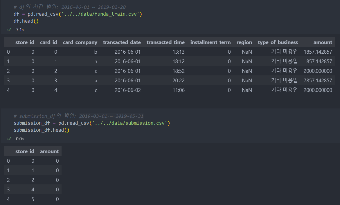
- 2019년 2월 28일까지의 약 3년의 카드 거래 데이터를 이용하여 2019년 3월 1일 ~ 5월 31일 상점별 3개월 총 매출 예측
데이터
funda_train.csv:
store_id: 상점 고유 id
card_id: 카드 고유 id
card_company: 비식별화된 카드회사
transcated_date: 거래 날짜
transacted_time: 거래 시간
installment_term: 할부 개월 수
region: 상점 지역
type_of_business: 상점 업종
amount: 거래액
submission.csv:
store_id: 상점 고유 id
문제
제공된 데이터의 레코드 단위는 '거래' -> 예측하고자 하는 레코드 단위는 3개월 간 상점 매출.
예측하고자 하는 데이터에 맞게 제공된 데이터를 새롭게 구축해야 할 필요성이 있다.
source code : GitHub
학습 데이터 구축
- 현재 데이터는 상점별/날짜별의 낱개 샘플들의 데이터
- 학습 데이터, 즉 월별(3개월) 매출 데이터의 예측을 위한 머신러닝 모델링을 위해 알맞는 학습 데이터 형식으로 만들어야 한다.
- raw data를 가지고 탐색하며 학습 데이터를 만들 특성들을 탐색하고 만든다.
레코드가 수집된 시간 기준으로 3개월 총 매출을 예측하도록 구조를 설계
시점 생성
제공 데이터는 총 33개월 기간을 가진다.
처음 시작 년의 월부터 마지막 년의 월까지 기간을 숫자로 지정한다.(계산 : (해당년 - 시작년) * 12(월) + 해당 월)
# .str.split을 이용한 년/월 추출
df['transacted_year'] = df['transacted_date'].str.split('-', expand = True).iloc[:, 0].astype(int)
df['transacted_month'] = df['transacted_date'].str.split('-', expand = True).iloc[:, 1].astype(int)

# 't'변수에 시작 월부터 수치화
df['t'] = (df['transacted_year'] - 2016) * 12 + df['transacted_month']
변수 탐색
1. 불필요한 특징 삭제
월별 기준은 숫자로 대체하였기에 날짜에 해당하는 컬럼과 card_id, card_company는 지나친 세분화가 될 수 있고 특징으로 유효할 가능성이 적다고 판단하여 삭제하도록 한다.
# 날짜 관련 특징 삭제
df.drop(['transacted_year', 'transacted_month', 'transacted_date', 'transacted_time'], axis = 1, inplace = True)

# card_id, card_company 삭제
df.drop(['card_id', 'card_company'], axis = 1, inplace = True)
2. 특징 탐색
주요 특징 3가지가 범주형 변수.
범주형이지만 지역, 업종의 상태 공간이 커서 더미화를 하기에는 부적절(ex. store(2000) * 지역(181) 이면 특징이 매우 커진다)
할부는 일시불(0)인지 할부(개월 수)인지 이진화
지역과 업종에 따른 매출 평균을 사용(결측치는 삭제하지 않고 문자로 변환해서 쓰기로 -> 모든 상점의 3개월 매출 예측인데 삭제하면 문제)
- 할부
- 지역
- 업종
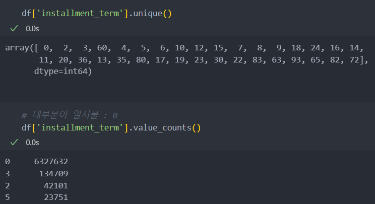
할부
할부 X(일시불) = 0
할부 = 개월 수
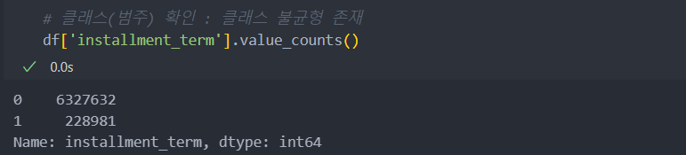
대부분이 할부인 것을 확인.
일시불과 할부를 0과 1로 변환하고 상점별 할부 현황을 파악.(상점들의 할부 현황이 매출에 영향을 미칠지 여부)
지역
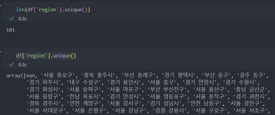
아래는 지역에 대한 정보다.
181개의 지역이 있고 결측치가 포함되어 있다.
결측치는 없음으로 설정하는데, 이유는 어떤 이유로 지역이 결측이 생겼을 이유 그리고 결측치를 삭제하였을 경우 해당하는 상점도 삭제가 될 수 있어 해당 상점에 대한 매출 예측이 어려울 수도 있기 때문이다.
결측치를 '없음'으로 채운다.
# 결측치 채우기
df['region'].fillna('없음', inplace = True)
업종
업종의 종류도 많고 결측치도 존재한다.
지역과 같이 결측치는 없음으로 설정한다.

# 결측치 채우기
df['type_of_business'].fillna('없음', inplace = True)
3. '월'(t) 기준 학습 데이터 생성
3개월 매출 예측이기에 월을 기준으로 매출 데이터가 필요.
중복을 제거하고, 각 상점별/월별 값에 평균 할부율/평균 매출을 추가하여 '월'별 학습 데이터를 생성한다.
'store_id', 'region', 'type_of_business' 3개의 컬럼은 동일하기에 't(월)'을 포함하여 4개의 컬럼의 중복을 제거.
중복을 제거한 데이터에, 할부율/월 매출 등 특징을 생성하여 추가할 것이다.
중복제거 및 평균 할부율 추가
# 중복 데이터 제거
df = df.drop_duplicates(subset=['store_id', 'region', 'type_of_business', 't'])[['store_id', 'region', 'type_of_business', 't']]

# 상점/월별 평균 할부율 추가
# installment_term_per_store : Series타입으로 상점별 평균 할부율
df['평균할부율'] = df['store_id'].replace(installment_term_per_store.to_dict())
해당 월별 이전 3개월 매출 추가
상점별 33개월의 모든 매출 정보가 있을까?(사정으로 인해 매출이 0이던가, 카드 사용 중지로 인해 누락된 월은 없는가?)
누락이 되었다면 상점별 월별 매출을 merge를 할 때 문제가 될 수 있다.
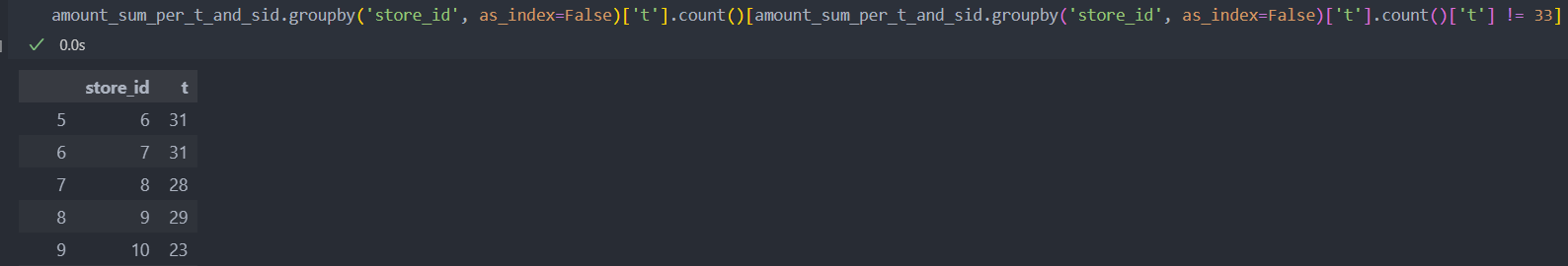
누락된 월이 있으니, pivot_table로 변환하여 NaN값이 된 매출을 처리하자.
누락된 월은 상점이 오픈을 하지 않았거나 사정에 의해 문을 닫아서 매출이 없는 경우를 생각해 볼 수 있다.
정확한 사정을 모르기에 NaN값으로 사용하기엔 부적절하여, 이전 달 혹은 다음 달의 매출과 비슷할 것이라 가정하고 결측치를 채운다.
amount_sum_per_t_and_sid = pd.pivot_table(df, values='amount', index='store_id', columns='t', aggfunc='sum')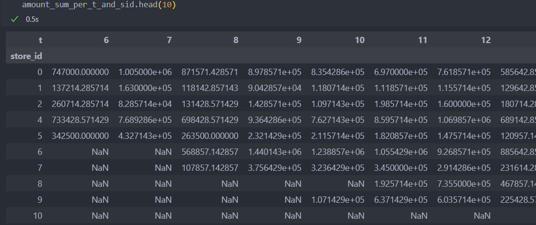
결측치가 있다면 앞의 월을 참조하고, 앞의 월이 없다면 다음 월을 참조하여 값을 채워넣는다.(fillna())
amount_sum_per_t_and_sid = amount_sum_per_t_and_sid.fillna(method='ffill', axis=1).fillna(method='bfill', axis=1)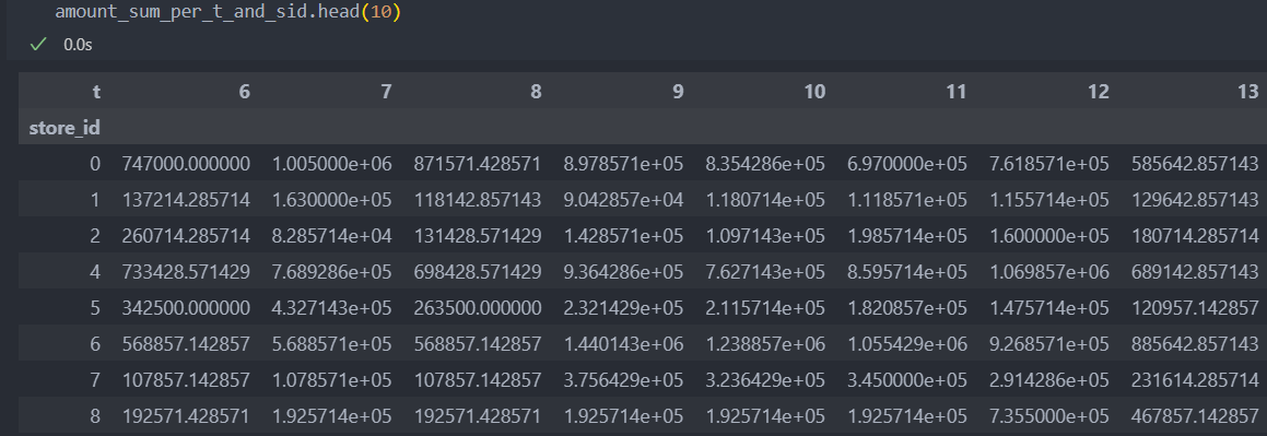
pivot은 옆으로 긴 열을 만들고, 반대로 stack는 아래로 긴 행을 만든다.
stack 함수를 사용하여 상점별 월별 매출을 넣어 데이터를 만든다.
amount_sum_per_t_and_sid = amount_sum_per_t_and_sid.stack().reset_index()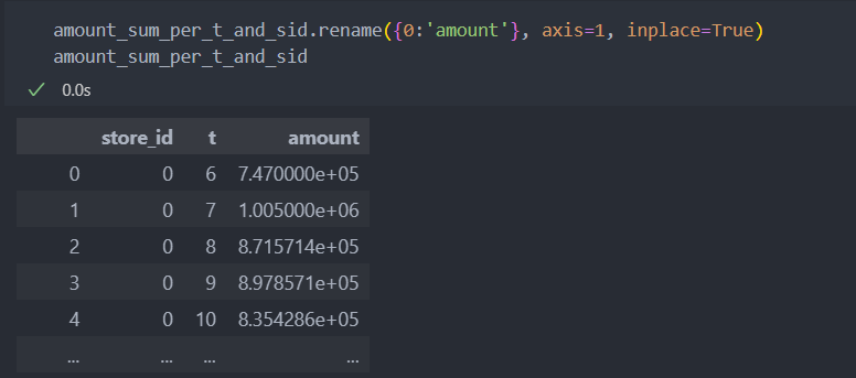
amount는 매출로 라벨 역할을 한다.
그래서 해당 매출이 아닌 해당 월의 이전 3개월 매출을 붙여서 현재 월의 매출을 예측하는 식으로 3개월의 매출을 예측하려 한다.
for k in range(1, 4):
    amount_sum_per_t_and_sid[f't_{k}'] = amount_sum_per_t_and_sid['t'] + k # 해당 월에 k(월)을 더해 1, 2, 3개월 앞의 데이터를 t_k로 컬럼 생성
    train_df = pd.merge(train_df, amount_sum_per_t_and_sid.drop('t', axis=1), left_on=['store_id', 't'], right_on=['store_id', f't_{k}'])

    # 추가한 뒤, 불필요한 변수 제거 및 변수명 변경
    train_df.rename({'amount':f'{k}_before_amount'}, axis=1, inplace=True)
    train_df.drop([f't_{k}'], axis=1, inplace=True)
    amount_sum_per_t_and_sid.drop([f't_{k}'], axis=1, inplace=True)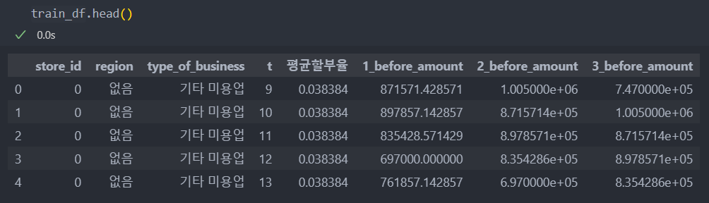
같은 방식으로 지역별/업종별 매출 합계의 평균도 추가해보자.
지역별 이전 3개월 매출의 평균 추가
# amount_sum_per_t_and_sid의 store_id를 region으로 대체시키기
store_to_region = df[['store_id', 'region']].drop_duplicates().set_index(['store_id'])['region'].to_dict() # 'key : store_id' : 'values : region'
amount_sum_per_t_and_sid['region'] = amount_sum_per_t_and_sid['store_id'].replace(store_to_region)

# 지역별 평균 매출 계산
amount_mean_per_t_and_region = amount_sum_per_t_and_sid.groupby(['region', 't'], as_index = False)['amount'].mean()

# 3개월 이전 매출 추가하는 방식과 일치
for k in range(1, 4):
    amount_mean_per_t_and_region[f't_{k}'] = amount_mean_per_t_and_region['t'] + k
    train_df = pd.merge(train_df, amount_mean_per_t_and_region.drop('t', axis=1), left_on=['region', 't'], right_on=['region', f't_{k}'])
    train_df.rename({'amount':f'{k}_before_amount_of_region'}, axis=1, inplace=True)

    train_df.drop([f't_{k}'], axis=1, inplace=True)
    amount_mean_per_t_and_region.drop([f't_{k}'], axis=1, inplace=True)
업종별 이전 3개월 매출의 평균 추가
# amount_sum_per_t_and_sid의 store_id를 type_of_business으로 대체시키기
store_to_type_of_business = df[['store_id', 'type_of_business']].drop_duplicates().set_index(['store_id'])['type_of_business'].to_dict() # 'key : store_id' : 'values : type_of_business'
amount_sum_per_t_and_sid['type_of_business'] = amount_sum_per_t_and_sid['store_id'].replace(store_to_type_of_business)

# 업종별 평균 매출 계산
amount_mean_per_t_and_type_of_business = amount_sum_per_t_and_sid.groupby(['type_of_business', 't'], as_index = False)['amount'].mean()

for k in range(1, 4):
    amount_mean_per_t_and_type_of_business[f't_{k}'] = amount_mean_per_t_and_type_of_business['t'] + k
    train_df = pd.merge(train_df, amount_mean_per_t_and_type_of_business.drop('t', axis=1), left_on=['type_of_business', 't'], right_on=['type_of_business', f't_{k}'])
    train_df.rename({'amount':f'{k}_before_amount_of_type_of_business'}, axis=1, inplace=True)

    train_df.drop([f't_{k}'], axis=1, inplace=True)
    amount_mean_per_t_and_type_of_business.drop([f't_{k}'], axis=1, inplace=True)
해당 월에서 3개월 매출 추가(라벨 추가)
해당 월에서 1, 2, 3개월 앞의 매출을 추가한다.
매출을 추가하는 방식과 같은데, 이젠 k를 더하는 것이 아닌 빼주면 된다.
1개월 후의 매출 라벨을 추가하는 방식은, 현재 해당 매출은 1, 2, 3개월을 뺀 이전 월의 예측(라벨) 매출로 추가한다.
for k in range(1, 4):
    amount_sum_per_t_and_sid[f't_{k}'] = amount_sum_per_t_and_sid['t'] - k # 현재 월 : t - k / k개월 후 예측 라벨 월 : t 월
    train_df = pd.merge(train_df, amount_sum_per_t_and_sid.drop('t', axis=1), left_on=['store_id', 't'], right_on=['store_id', f't_{k}'])
    train_df.rename({'amount':f'Y_{k}'}, axis=1, inplace=True)

    train_df.drop([f't_{k}'], axis=1, inplace=True)
    amount_sum_per_t_and_sid.drop([f't_{k}'], axis=1, inplace=True)

# 3개월 매출 합계 라벨
train_df['Y'] = train_df['Y_1'] + train_df['Y_2'] + train_df['Y_3']
학습 데이터 탐색 및 전처리
이제 학습 데이터를 생성했다.
이 데이터를 바탕으로 데이터 분할, 이상치 제거, 스케일링 등의 전처리 작업을 진행한다.
특징/라벨, 학습/평가 데이터 분리 및 탐색
먼저 특징과 라벨을 분리하고 학습/평가 데이터로 분리한다.
# 특징(필요없는 컬럼과 라벨 삭제)
X = train_df.drop(['store_id', 'region', 'type_of_business', 't', 'Y_1', 'Y_2', 'Y_3', 'Y'], axis = 1)
Y = train_df['Y']
from sklearn.model_selection import train_test_split
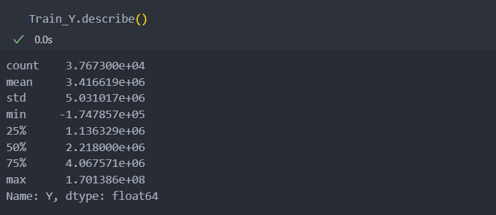
Train_X, Test_X, Train_Y, Test_Y = train_test_split(X, Y) # default : test_size = 0.25로 사용한다.라벨 변수의 분포를 살펴보자.
아래와 같이 스케일의 차이가 매우 큰 것을 알 수 있고, IQR 75%에 비해 최대값이 너무 크고 최소값은 0으로 차이들이 매우 큰 것을 확인할 수 있다.
예측 모델에서는 이상치가 매우 튀는 값이 있을 경우 안정적인 분석이 힘들 수 있으므로,
라벨을 확인하여 이상치를 제거한다.
스케일의 차이가 많으므로 스케일링도 진행한다.
이상치 제거
IQR을 벗어나는 이상치를 제외한 데이터만 학습 데이터로 쓰기 위한 함수를 작성한다.
def IQR_rule(data):
    # IQR 계산
    Q1 = np.quantile(data, 0.25)
    Q3 = np.quantile(data, 0.75)
    IQR = Q3 - Q1

    # IQR에서 outlier이 아닌 데이터들의 인덱스들의 bool타입을 list로 반환
    not_outlier_condition = (Q3 + 1.5 * IQR > data) & (Q1 - 1.5 * IQR < data)

    return not_outlier_condition

# 이상치가 아닌 데이터들의 인덱스 리스트
Y_condition = IQR_rule(Train_Y)

# 이상치가 아닌 데이터만 다시 학습 데이터로 추림
Train_Y = Train_Y[Y_condition]
Train_X = Train_X[Y_condition]
치우치는 값 제거
아래와 같이 skew()의 값들이 모두 양수로써, 모든 값들이 왼쪽으로 치우쳐 있음이 확인된다.
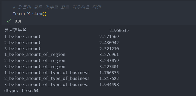
왜도의 절대값 1.5 이상이 되는 값들은 보통 치우친 값이라고 판단하고 루트를 사용하여 치우침을 완화시킨다.
# 1.5 이상인 컬럼 가져오기 : 사실 모든 컬럼이 치우쳐 있다.
biased_variables = Train_X.columns[Train_X.skew().abs() > 1.5]

# 치우침을 제거하기 위해 루트를 적용하여 완화시킨다.
Train_X[biased_variables] = Train_X[biased_variables] - Train_X[biased_variables].min() + 1 # 루트를 사용하기 위해 : 기존 값 - 최소값 + 1
Train_X[biased_variables] = np.sqrt(Train_X[biased_variables]) # 루트 사용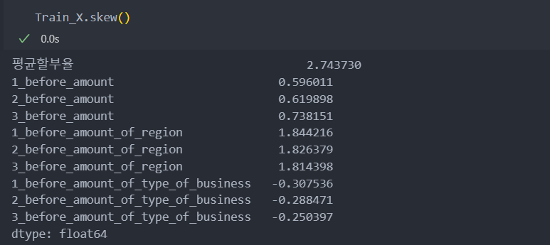
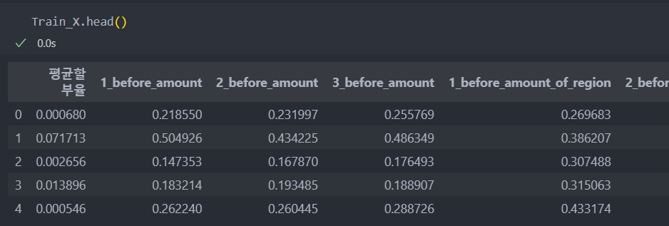
스케일링
특징들의 값의 스케일에 차이가 있으면 작은 값들은 예측을 하는데 영향을 주지 못하는 경향이 있다.
그래서 값들의 정규화를 위해 minmax scaling을 진행한다.
from sklearn.preprocessing import MinMaxScaler
# 스케일러 인스턴스 및 학습
scaler = MinMaxScaler().fit(Train_X)

# 적용
s_Train_X = scaler.transform(Train_X)
s_Test_X = scaler.transform(Test_X)

# 스케일러의 반환 값은 array형식 -> 다시 DataFrame 형식으로
Train_X = pd.DataFrame(s_Train_X, columns=Train_X.columns)
Test_X = pd.DataFrame(s_Test_X, columns=Train_X.columns)
모델에 넣기 전 최종 데이터
모델링
참조 : 특징 선택
특징 대비 샘플 수가 많고, 특징을 모두 연속형으로 되어 있다.
사용할 모델
- kNN model
- RandomForestRegressor model
- LightGBM model
특징 선택
- 특징 선택 : 3 ~ 10개 사용
- 통계량 : F 통계량 / 연속형 변수들이며 회귀 -> f_regression 사용
모델 선정 및 하이퍼 파라미터 튜닝
모델 선정
# 모델
from sklearn.neighbors import KNeighborsRegressor as KNN
from sklearn.ensemble import RandomForestRegressor as RFR
from lightgbm import LGBMRegressor as LGB

# score 및 통계량, 파라미터 튜닝
from sklearn.model_selection import ParameterGrid
from sklearn.metrics import mean_absolute_error as MAE
from sklearn.feature_selection import *
하이퍼 파라미터 튜닝
각 모델의 각 튜닝별로 iteration은 수는 512개이다.
# 하이퍼 파라미터를 담을 변수 생성
param_grid = dict()

# 모델별 하이퍼 파라미터 그리드 생성
param_grid_for_knn = ParameterGrid({
                                    'n_neighbors':[1, 3, 5, 7],
                                    'metric':['euclidean', 'cosine']
})
param_grid_for_RFR = ParameterGrid({
                                    'max_depth':[2, 3, 4, 5],
                                    'n_estimators':[100, 200],
                                    'max_samples':[0.5, 0.6, 0.7, None]
})
param_grid_for_LGB = ParameterGrid({
                                    'max_depth':[2, 3, 4, 5],
                                    'n_estimators':[100, 200],
                                    'learning_rate':[0.05, 0.1, 0.15]
})

param_grid[KNN] = param_grid_for_knn
param_grid[RFR] = param_grid_for_RFR
param_grid[LGB] = param_grid_for_LGB
학습 진행
best_score = 1e9
iteration_num = 0
knn_list = []
rfr_list = []
lgb_list = []
for k in range(10, 2, -1): # 메모리 부담을 줄이기 위한
selector = SelectKBest(f_regression, k=k).fit(Train_X, Train_Y)
selected_features = Train_X.columns[selector.get_support()]
# 선택한 특징으로 학습 진행하기 위한 : 특징 개수를 줄여나가며 메모리 부담도 줄인다.
Train_X = Train_X[selected_features]
Test_X = Test_X[selected_features]
for m in param_grid.keys():
for p in param_grid[m]:
model = m(**p).fit(Train_X.values, Train_Y.values)
pred = model.predict(Test_X.values)
score = MAE(Test_Y.values, pred)
if score < best_score:
best_score = score
best_model = m
best_parameter = p
best_features = selected_features
if m == KNN:
knn_list.append(score)
elif m == RFR:
rfr_list.append(score)
elif m == LGB:
lgb_list.append(score)
iteration_num += 1
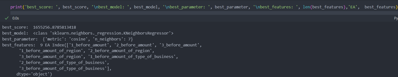
print(f'iter_num-{iteration_num}/{max_iter_num} => score : {score:.3f}, best score : {best_score:.3f}')best score, model, param, features를 보자.
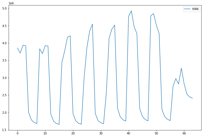
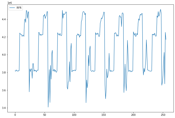
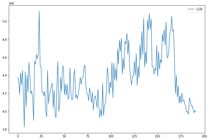
학습이 끝난 모델별 점수를 라인 그레프로 각각 그려보자.
점수가 낮을 수록 좋다.
최종 모델 및 파라미터 학습
best score, model, param, features를 가지고 최종 모델을 선정 및 학습을 한다.
def pipeline(X):
    X[biased_variables] = X[biased_variables] - X[biased_variables].min() + 1
    X[biased_variables] = np.sqrt(X[biased_variables]) # 치우침 제거
    X = pd.DataFrame(scaler.transform(X), columns = X.columns) # 스케일링
    X = X[best_features] # best_features 적용
    return X

model = best_model(**best_parameter).fit(pipeline(X).values, Y)
적용 데이터 구성
제공된 데이터(funda_train.csv)의 store_id와 제출해야 하는 데이터(submission.csv)의 store_id를 보면 제공되는 데이터보다 제출해야 하는 데이터의 store_id가 많지는 않을 것이다. 제출해야 하는 데이터의 store_id가 더 많다면 추가된 store_id는 분석이 어렵기 때문이다.
제출해야 하는 데이터에 맞춰 제출을 해야하기에, store_id를 바탕으로 이전의 제공된 데이터를 전처리한 과정을 제출해야 하는 데이터에 적용시켜서 최종 모델로 학습을 진행해야 한다.
특징 추가
submission_df에 대해서도 같은 전처리 과정을 통해 처리를 한다.
기본 컬럼 월('t')와 지역, 업종을 추가한다.
# 현재 월('t')까지(2월) 추가 -> 현재 월을 기준으로 3개월 예측 : 2019-03-01 ~ 2019-05-31
submission_df['t'] = (2019 - 2016) * 12 + 2

# region 변수와 type_of_business 변수 추가
submission_df['region'] = submission_df['store_id'].replace(store_to_region)
submission_df['type_of_business'] = submission_df['store_id'].replace(store_to_type_of_business)
그리고 submission_df의 store_id 및 컬럼에 맞춰 전처리한 결과를 똑같이 붙여준다.
# 평균할부율 추가
submission_df['평균할부율'] = submission_df['store_id'].replace(installment_term_per_store.to_dict())
# 1, 2, 3개월 이전 매출 데이터 추가
for k in range(1, 4):
amount_sum_per_t_and_sid['t_{}'.format(k)] = amount_sum_per_t_and_sid['t'] + k
submission_df = pd.merge(submission_df, amount_sum_per_t_and_sid.drop('t', axis = 1), left_on = ['store_id', 't'], right_on = ['store_id', 't_{}'.format(k)])
submission_df.rename({"amount":"{}_before_amount".format(k)}, axis = 1, inplace = True)
submission_df.drop(['t_{}'.format(k)], axis = 1, inplace = True)
amount_sum_per_t_and_sid.drop(['t_{}'.format(k)], axis = 1, inplace = True)
# 1, 2, 3개월 이전 지역별 매출 평균 데이터 추가
for k in range(1, 4):
amount_mean_per_t_and_region['t_{}'.format(k)] = amount_mean_per_t_and_region['t'] + k
submission_df = pd.merge(submission_df, amount_mean_per_t_and_region.drop('t', axis = 1), left_on = ['region', 't'], right_on = ['region', 't_{}'.format(k)])
submission_df.rename({"amount":"{}_before_amount_of_region".format(k)}, axis = 1, inplace = True)
submission_df.drop(['t_{}'.format(k)], axis = 1, inplace = True)
amount_mean_per_t_and_region.drop(['t_{}'.format(k)], axis = 1, inplace = True)
# 1, 2, 3개월 이전 업종별 매출 평균 데이터 추가
for k in range(1, 4):
amount_mean_per_t_and_type_of_business['t_{}'.format(k)] = amount_mean_per_t_and_type_of_business['t'] + k
submission_df = pd.merge(submission_df, amount_mean_per_t_and_type_of_business.drop('t', axis = 1), left_on = ['type_of_business', 't'], right_on = ['type_of_business', 't_{}'.format(k)])
submission_df.rename({"amount":"{}_before_amount_of_type_of_business".format(k)}, axis = 1, inplace = True)
submission_df.drop(['t_{}'.format(k)], axis = 1, inplace = True)
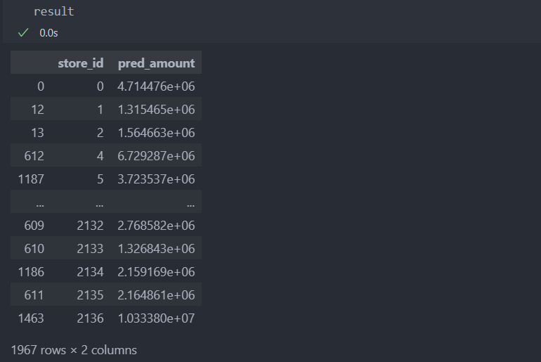
amount_mean_per_t_and_type_of_business.drop(['t_{}'.format(k)], axis = 1, inplace = True) 결과 도출
최종 모델로 결과 도출하기.
# 모델에 들어갈 features
submission_X = submission_df[X.columns]
submission_X = pipeline(submission_X)

# 예측
pred_Y = model.predict(submission_X)

# 제출 DataFrame 형식으로
result = pd.DataFrame({"store_id":submission_df['store_id'].values,
                      "pred_amount":pred_Y})

# 상점 id 순으로
result.sort_values(by='store_id', inplace=True)