
문제 정의
신용 데이터를 활용하여 사기 거래로 인한 고객 클레임 및 고객 탈퇴 등을 미연에 방지하고자 한다.
데이터 확인
소스 코드 : GitHub
데이터 특징
- numeric/categorical data로 구분
- 데이터 샘플도 많고 특징도 많은 데이터
- 결측치가 존재
- 사기 거래 예측 문제 답게 클래스 불균형 문제가 심각(전체 데이터에서 사기 거래 약 5%)
- 데이터 features
해당 도메인 지식이 있어야 깊게 데이터를 확인해 볼 수 있을 것이라 판단되며, 사기 거래에 대한 중요 특징을 통해서 중저마 관리를 해야할 필요성이 있음.
| account_age_days | transaction_amt | transaction_adj_amt | historic_velocity | ip_address | user_agent |
|---|---|---|---|---|---|
| 계좌 생성후 지난일 | 거래금액 | 거래 조정 금액 | 과거 거래금액 | IP주소 | 사용환경 |
| email_domain | phone_number | billing_city | billing_postal | billing_state | card_bin |
|---|---|---|---|---|---|
| email 도메인 | 전화번호 | 청구도시 | 청구우편번호 | 청구주 | 카드bin번호(앞6자리) |
| currency | cvv | signature_image | transaction_type | transaction_env | EVENT_TIMESTAMP |
|---|---|---|---|---|---|
| 통화 | CVV | 서명이미지 | 거래종류 | 거래환경 | 거래일자 |
| billing_address | merchant_id | locale | tranaction_initiate | days_since_last_logon | inital_amount |
|---|---|---|---|---|---|
| 청구주소 | 상점ID | 지역 | 거래초기코드 | 마지막로그인후경과일 | 초기잔액 |
| EVENT_LABEL |
|---|
| 사기여부 |
데이터 EDA & 전처리
기본 데이터 확인
데이터 샘플도 많고 특징도 많다.
df.shape
>
(150000, 26)
수치형 데이터와 문자형 데이터가 섞여 있다.
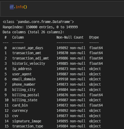
결측치가 있는데, 많지 않은 관계로 삭제하기로 한다.
df.isnull().sum()
>
account_age_days         108
transaction_amt          130
transaction_adj_amt      114
historic_velocity        115
ip_address               127
user_agent               113
email_domain              90
phone_number             127
billing_city             116
billing_postal           124
billing_state            113
card_bin                 128
currency                 108
cvv                      123
signature_image          105
transaction_type         116
transaction_env          123
EVENT_TIMESTAMP          112
applicant_name           143
billing_address          134
merchant_id              107
locale                   134
tranaction_initiate      126
days_since_last_logon    136
inital_amount            128
EVENT_LABEL                0
dtype: int64

# 결측치 삭제
# 결측치의 개수가 적어서 삭제를 진행하기로 한다. - 3천개의 데이터 삭제
df = df.dropna(axis=0)

df.shape
>
(147000, 26)
사기 거래에 대한 데이터답게 클래스 불균형이 심각한다.
# 클래스 불균형 심각
df['EVENT_LABEL'].value_counts()
>
legit    138996
fraud      8004

# 사기 비율
# 5% 정도가 사기 거래
df['EVENT_LABEL'].value_counts()[1] / len(df) * 100
>
5.444897959183673
user_agent 특징은 브라우저의 정보만 담기로 한다.
# user_agent 특징에서 브라우저 name만 선택해서 진행
df['user_agent'] = df['user_agent'].apply(lambda x: x.split('/')[0])
변수 탐색
변수의 유니크값 확인.
for col in df.columns:
    print(f'{col} - nums : {len(df[col].unique())} EA')
    print(f'{df[col].unique()}')
    print('_'*40)
데이터가 수치형인지 문자형인지에 따라서 numeric 변수와 categorical 변수로 나눈다.
numeric_lists, categorical_lists = [], []

for col in df.columns:
    if df[col].dtypes == 'O':
        categorical_lists.append(col)
    else:
        numeric_lists.append(col)
숫자형 데이터라고 해서 반드시 연속형 변수는 아니기에, 특징의 unique값 등을 세세하게 확인하는 작업이 필요하다.
연속형 변수 탐색
연속형 변수들을 그룹으로 묶어 범주화시켜보자.
특히 금액과 관련된 변수에 대해서 확인하고 그룹화하여 사기 비율을 확인한다.
거래 금액이 클 수록 사기 거래 비율이 늘어난다.
plt.figure(figsize=(12, 8))
sns.distplot(df['transaction_amt'])
plt.show()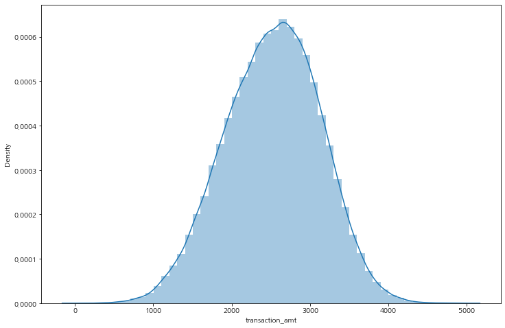
df['transaction_amt_gp'] = np.where(df['transaction_amt'] <= 2000, 1,
                                    np.where(df['transaction_amt'] <= 3000, 2, 3))

# 평균 사기 5% -> 그룹 1, 2, 3 사기 비율이 다르다 : 거래 금액이 클수록 사기 거래 비율이 늘어난다
gp1_3 = df.groupby(['transaction_amt_gp', 'EVENT_LABEL'], as_index=False)['transaction_amt'].count()
print(f'gp 1 : {gp1_3.iloc[0, -1] / (gp1_3.iloc[0, -1] + gp1_3.iloc[1, -1])}')
print(f'gp 2 : {gp1_3.iloc[2, -1] / (gp1_3.iloc[2, -1] + gp1_3.iloc[3, -1])}')
print(f'gp 3 : {gp1_3.iloc[4, -1] / (gp1_3.iloc[4, -1] + gp1_3.iloc[5, -1])}')
>
gp 1 : 0.011856379941557787
gp 2 : 0.057159442266001684
gp 3 : 0.08612177729018101
거래 조정 금액은 금액이 적을 수록 비율이 늘어나는 것이 확인된다.
그 비율은 상당히 큰 영향을 미칠 것이라 판단이 된다.
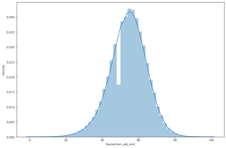
df['transaction_adj_amt_gp'] = np.where(df['transaction_adj_amt'] <= 30, 1,
                                    np.where(df['transaction_adj_amt'] <= 60, 2, 3))

# 평균 사기 5% -> 그룹 1, 2, 3 사기 비율이 다르다 : 거래 조정 금액이 작을 수록 사기 거래 비율이 늘어난다
gp1_3 = df.groupby(['transaction_adj_amt_gp', 'EVENT_LABEL'], as_index=False)['transaction_amt'].count()
print(f'gp 1 : {gp1_3.iloc[0, -1] / (gp1_3.iloc[0, -1] + gp1_3.iloc[1, -1])}')
print(f'gp 2 : {gp1_3.iloc[2, -1] / (gp1_3.iloc[2, -1] + gp1_3.iloc[3, -1])}')
print(f'gp 3 : {gp1_3.iloc[4, -1] / (gp1_3.iloc[4, -1] + gp1_3.iloc[5, -1])}')
>
gp 1 : 0.7248293515358362
gp 2 : 0.057234064657492846
gp 3 : 0.006318504190844616
과거의 거래 금액은 현재 사기 거래에 대한 유의미한 데이터로 보기 힘들다.
# 평균 사기 5% -> 과거 거래 금액은 모두 비슷한 비율을 보이는 것으로 보아, 유의미한 데이터로 보기 힘들다.
gp1_3 = df.groupby(['historic_velocity_gp', 'EVENT_LABEL'], as_index=False)['transaction_amt'].count()
print(f'gp 1 : {gp1_3.iloc[0, -1] / (gp1_3.iloc[0, -1] + gp1_3.iloc[1, -1])}')
print(f'gp 2 : {gp1_3.iloc[2, -1] / (gp1_3.iloc[2, -1] + gp1_3.iloc[3, -1])}')
print(f'gp 3 : {gp1_3.iloc[4, -1] / (gp1_3.iloc[4, -1] + gp1_3.iloc[5, -1])}')
>
gp 1 : 0.05491260084517864
gp 2 : 0.05385470105676257
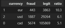
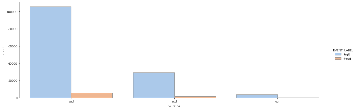
gp 3 : 0.055941023417172595범주형 변수 탐색
카테고리 범주형 변수는 함수를 만들어서 변수에 따른 합법/사기 비율을 확인해보자.
범주별로 유의미한 데이터도 있고 그렇지 않은 데이터가 섞여 있으니 하나하나 들여다볼 필요성이 있다.
def get_category_ratio(cat_val):
    df_cat_val = df.groupby([cat_val, 'EVENT_LABEL'], as_index=False)['EVENT_TIMESTAMP'].count()

    pivot_cat_val = pd.pivot_table(df_cat_val, index=cat_val, columns='EVENT_LABEL', values='EVENT_TIMESTAMP').reset_index()
    pivot_cat_val.columns.names=['']

    pivot_cat_val['ratio'] = round((pivot_cat_val.iloc[:, 1] / (pivot_cat_val.iloc[:, 1] + pivot_cat_val.iloc[:, 2])) * 100, 1)
    pivot_cat_val.sort_values(by='ratio', ascending=False, inplace=True)

    return pivot_cat_val

# 탐색할 카테고리
col_idx = 'currency'
# 비율 확인
get_category_ratio(col_idx)
# catplot 그려보기
plt.figure(figsize=(20, 8))
sns.catplot(data=df, x=col_idx, hue='EVENT_LABEL', kind='count', palette='pastel', edgecolor='.6' , aspect=3)
plt.show()
ex)
모델링
연속형과 범주형이 섞여 있고 샘플도 많고 특징도 많다. 그래서 모델은 Tree 기반의 앙상블 모델 RandomForestClassifier와 트리 기반의 부스팅 방식인 LGBMClassifier를 사용하도록 하며, 평가지표는 f1 score를 사용한다.
데이터 나누기
label data를 수치형으로 바꾸고 학습/평가 데이터로 분리한다.
# label data 수치형으로 변환 후 데이터 분리
df['EVENT_LABEL'] = np.where(df['EVENT_LABEL']=='fraud', 1, 0)
df['EVENT_LABEL'].value_counts()

X = df.drop(['EVENT_TIMESTAMP', 'EVENT_LABEL', 'transaction_amt_gp'], axis=1)
Y = df['EVENT_LABEL']

train_x, test_x, train_y, test_y = train_test_split(X, Y, stratify=Y)

train_x.shape, train_y.shape, test_x.shape, test_y.shape
>
((110250, 26), (110250,), (36750, 26), (36750,))
LabelEncoder
특징들을 살펴보고 필요한 데이터를 남긴 후 LabelEncoder를 진행한다.
for col in categorical_lists:
    le = LabelEncoder()
    le.fit(list(train_x[col]) + list(test_x[col]))
    train_x[col] = le.transform(train_x[col])
    test_x[col] = le.transform(test_x[col])
하이퍼 파라미터
model_param_dict = {}
rfc_param_grid = ParameterGrid({
                                'max_depth':[3, 5, 10, 15, 30, 50],
                                'n_estimators':[100, 200, 400, 800],
                                'random_state':[29, 1000],
                                'n_jobs':[-1]
})
lgbm_param_grid = ParameterGrid({
                                'max_depth':[3, 5, 10, 15, 30, 50],
                                'n_estimators':[100, 200, 400, 800],
                                'learning_rate':[0.05, 0.1, 0.2]
})

model_param_dict[RFC] = rfc_param_grid
model_param_dict[LGBM] = lgbm_param_grid
학습 및 모델 선정
best_score = -1
num_iter = 0

for m in model_param_dict.keys():
    for p in model_param_dict[m]:
        model = m(**p).fit(train_x.values, train_y.values)
        pred = model.predict(test_x.values)
        score = f1_score(test_y.values, pred)

        if score > best_score:
            best_score = score
            best_model = m
            best_param = p

        num_iter += 1

        print(f'iter : {num_iter}/{max_iter} | best score : {best_score:.3f}')
최종 모델 선정
# 모델
best_model
>
lightgbm.sklearn.LGBMClassifier
# 파라미터
best_param
>
{'learning_rate': 0.1, 'max_depth': 15, 'n_estimators': 800}
최종 모델 평가 확인하면 과적합 경향이 조금 보이나, 평가 데이터의 수치도 좋아서 사용하기로 한다.
classification report
model = best_model(**best_param)
model.fit(train_x, train_y)

train_pred = model.predict(train_x)
test_pred = model.predict(test_x)

print(classification_report(train_y, train_pred))
print(classification_report(test_y, test_pred))
>
              precision    recall  f1-score   support

           0       1.00      1.00      1.00    104247
           1       1.00      1.00      1.00      6003

    accuracy                           1.00    110250
   macro avg       1.00      1.00      1.00    110250
weighted avg       1.00      1.00      1.00    110250

              precision    recall  f1-score   support

           0       0.99      1.00      0.99     34749
           1       0.94      0.75      0.83      2001

    accuracy                           0.98     36750
   macro avg       0.96      0.87      0.91     36750
weighted avg       0.98      0.98      0.98     36750
roc acu score
train_proba = model.predict_proba(train_x)[:, 1]
test_proba = model.predict_proba(test_x)[:, 1]

train_score = roc_auc_score(train_y, train_proba)
test_score = roc_auc_score(test_y, test_proba)

print('train roc_auc score :', train_score)
print('test roc_auc score : ', test_score)
>
train roc_auc score : 0.9999998897402047
test roc_auc score :  0.95443831797877
특징들 중 모델에 영향을 많이 미친 순서대로 bar 플롯으로 확인해보자.
ftr_importances_values = model.feature_importances_
ftr_importance = pd.Series(ftr_importances_values, index=train_x.columns)
ftr_top = ftr_importance.sort_values(ascending=False)

plt.figure(figsize=(12, 8))
plt.title('Feature Importances')
sns.barplot(x=ftr_top, y=ftr_top.index)
plt.show()
기대 효과
사기 거래 제한으로 인해 고객 클레임 및 탈퇴를 방지, 감소 방어