문제 정의

Bosch사의 조립 공정 라인의 모든 단계에 대한 데이터를 분석하여,
제품의 불량을 예측한다.

데이터 확인

출처 : kaggle

소스코드 : GitHub

제공된 데이터의 특징

• numeric/categorical data로 구분
• 데이터샘플은 적고 특징(컬럼)이 굉장히 많은 데이터로써 특징 추출이 매우 중요한 문제
• 결측치가 매우 많다.
• 비식별화된 특징이 매우 많다
• 불량 예측문제 답게 클래스 불균형 문제가 심각
• 독립된 ID별 - L(제조 라인)_S(제조 스테이션)_F(기능 번호)
  - ID 100이 10번 제조 라인에서 생산될 시, 다른 제조 라인은 모두 결측치가 될 수 밖에 없는 구조

EDA & 전처리

수치형과 범주형 데이터를 'Id'를 index로 하여 각각 탐색 및 전처리를 진행하고 통합하기로 한다.

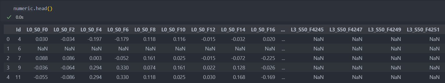
수치형 데이터

먼저 'Id'를 index로 하고 라벨 데이터를 분리한 후 진행한다.

df = numeric.copy()

df.set_index('Id', inplace=True)

X = df.drop('Response', axis=1)
Y = df['Response']

'Id'별로 거쳐간 공정을 확인하고 라인 혹은 스테이션이나 특징별로 데이터를 정리한 후,
'Id'별 데이터 값들의 통계량을 확인한다.
그리고 'Id'를 기준으로 공정 데이터들과 통계량 데이터들을 합칠 것이다.

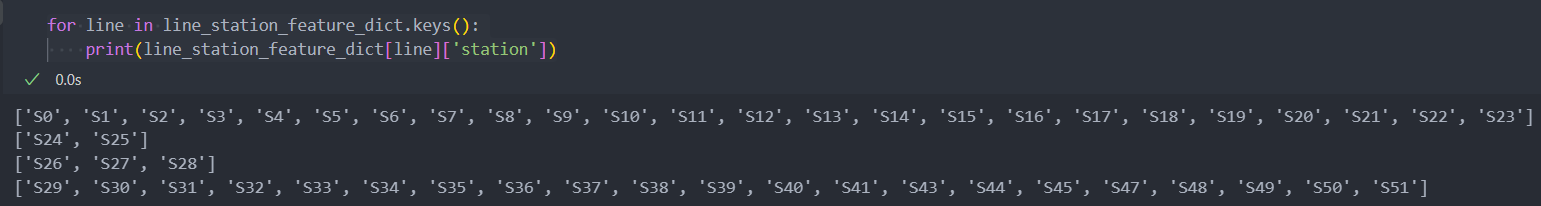
라인별 스테이션과 특징 확인

라인은 'L0-L3'까지 총 4개의 라인이 존재하며, 각 라인별 스테이션과 특징들을 담을 수 있도록 dict()자료형을 생성한다.

# dict()형 자료 생성
line_station_feature_dict = dict()

# 라인별 정보
line_station_feature_dict['L0'] = {'station':[], 'feature':[]}
line_station_feature_dict['L1'] = {'station':[], 'feature':[]}
line_station_feature_dict['L2'] = {'station':[], 'feature':[]}
line_station_feature_dict['L3'] = {'station':[], 'feature':[]}

그리고 각 라인별로 station, feature를 각각 중복없이 값을 입력하기 위해, 반복문을 통해서 데이터를 입력하도록 한다.
현재 X의 컬럼은 id는 index로 라벨 데이터는 분리하였기에, line-station-feature 정보만 있다.

for col in X.columns:
    line, station, feature = col.split('_') # _ 언더바를 기준으로 분리되어 있다.

    if station not in line_station_feature_dict[line]['station']:
        line_station_feature_dict[line]['station'].append(station)
    
    if feature not in line_station_feature_dict[line]['feature']:
        line_station_feature_dict[line]['feature'].append(feature)

이제 라인별 스테이션과 특징들을 확인해보자.

라인별 '스테이션'

라인별 '특징'

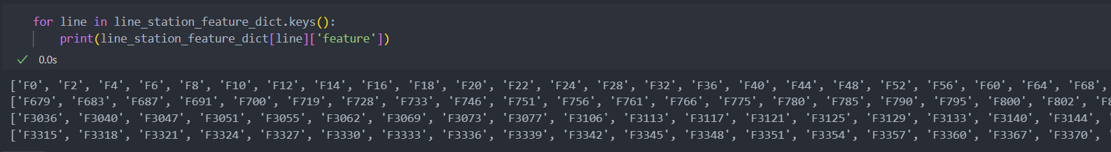
라인별로 데이터를 정리하기엔 라인이 4개이기에 너무 적고, 특징은 너무 많다.
그래서 라인별 '스테이션'으로 데이터를 정리하기로 한다.

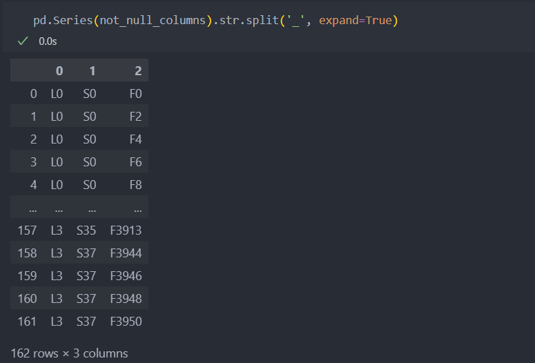
데이터의 index별(index가 'Id')로 결측치가 아닌 컬럼만 추출하여 사용한다.

# index별 결측이 아닌 컬럼이 공정이라고 판단, 그 컬럼만 사용
not_null_columns = X.columns[X.iloc[0].notnull()] # 첫번째만 확인.

pd.Series(not_null_columns).str.split('_', expand=True)

첫번째 'Id'의 제품이 거쳐간 라인과 스테이션 그리고 특징들이다.

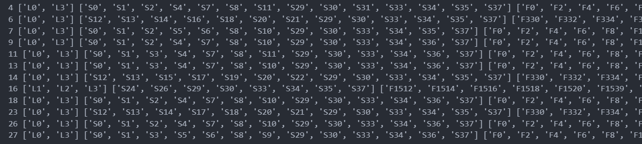
이런 방식으로 결측치가 아닌 데이터들의 'Id'별 거쳐간 라인과 스테이션, 특징들을 10개만 확인해보자.

먼저,
iterrows()를 사용하여 모든 'Id'별로 순회하면서 확인한다.
Id는 index로 설정하였기에, idx가 제품 'Id'이고 그 제품의 모든 행이 결측치가 아니라면 공정을 거친 것이라 판단된다.
그래서 결측치가 아닌 컬럼을 각각의 라인과 스테이션 그리고 특징별로 리스트로 묶어서 확인한다.

num_iter = 0

for idx, row in X.iterrows():
    if sum(row.notnull()) > 0:
        not_null_columns = X.columns[row.notnull()] # 모든 컬럼 중 결측치가 아닌 컬럼만 가져와서
        
        # 각 공정별로 확인하여 데이터 확인
        lines = pd.Series(not_null_columns).str.split('_', expand=True).iloc[:, 0].drop_duplicates().to_list()
        stations = pd.Series(not_null_columns).str.split('_', expand=True).iloc[:, 1].drop_duplicates().to_list()
        features = pd.Series(not_null_columns).str.split('_', expand=True).iloc[:, 2].drop_duplicates().to_list()

        print(idx, lines, stations, features)

        if num_iter > 10:
            break
    num_iter += 1

데이터를 전처리 할 때에는 특징은 제외하고 스테이션까지 하기로 한다.

'Id'별 거쳐간 라인과 스테이션 그리고 특징들이다.
아래는 제품 'Id'별로 라인은 같은 라인의 공정이지만 스테이션이 각각 다른 것을 볼 수 있다.
이것이 불량을 확인하는데 있어 중요한 변수가 될 것이라 예상한다.

'Id'별 거쳐간 스테이션 확인

제품 'Id'별 거쳐간 스테이션 데이터를 정리해보자.

'Id'별로 거쳐간 스테이션은 각각 다르기 때문에 데이터를 통합할 때 어려움이 있다.
그래서 모든 스테이션 중에서 'Id'별 거쳐간 스테이션이라면 1로 아니면 0으로 데이터를 정리한다.

모든 스테이션의 집합을 리스트로 정리한다.

total_stations = []

for line in line_station_feature_dict.keys():
    total_stations += line_station_feature_dict[line]['station'] # 라인별 스테이션이 모두 다르다는 것은 위에서 이미 확인을 하였다.

모든 제품 'Id'별 거쳐간 스테이션을 정리한다.

station_x = []

for idx, row in X.iterrows():
    if sum(row.notnull()) == 0:
        station_x.append(np.zeros(len(total_stations))) # 공정을 거치지 않은 데이터도 포함시켜야 한다.
    
    else:
        not_null_columns = X.columns[row.notnull()] # 결측치가 아닌 컬럼만 선별
        stations = pd.Series(not_null_columns).str.split('_', expand=True).iloc[:, 1].drop_duplicates().to_list() # 결측치가 아닌 컬럼 리스트, 스테이션별 특징으로 인해 중복이 되었다면 중복을 제거하여 스테이션만 남긴다.
        station_x.append(np.isin(total_stations, stations)) # 모든 station별로 True/False

station_x = pd.DataFrame(station_x, index=X.index, columns=total_stations)
station_x = station_x.astype(int) # True = 1, False = 0 변환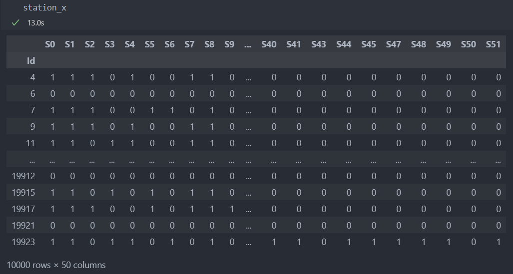

통계량 확인

순서대로 진행하는 공정에서 제품별 서로 다른 공정의 길이를 거치기에 공통적인 데이터를 분류해야 한다.
그래서 time series와 같은 시계열에서 통계량의 추출은 '길이가 다른 시계열'을 분류할 때 자주 사용이 된다.

이상치, 결측치를 처리하는 함수와 각 'Id'별 대표 통계량들을 반환하는 함수를 생성한다.

이상치 처리 함수

def remove_outliers(val, w=1.5):
    Q1 = np.quantile(val, 0.25)
    Q3 = np.quantile(val, 0.75)
    IQR = Q3 - Q1

    low_cond = Q1 - w * IQR < val
    high_cond = Q3 + w * IQR > val
    total_cond = np.logical_and(low_cond, high_cond)

    return val[total_cond]

결측치 및 통계량 반환 함수 : 평균, 분산, 최대값, 최소값, 첨도, 제곱평균제곱근 - time series에서 자주 사용되는 대표 통계량

def extract_statistical_feature(val): # val : Id별
    if val.notnull().sum() == 0:
        return pd.Series([0] * 6)
    else:
        val = val.copy().dropna() # 결측치 저리
        val = remove_outliers(val) # 이상치 처리

        val_mean = val.mean() # 평균
        val_var = val.var() # 분산
        val_max = val.max() # 최대값
        val_min = val.min() # 최소값
        val_kurtosis = stats.kurtosis(val) # 첨도
        val_rms = np.sqrt(sum(val**2 / len(val))) # 제곱평균제곱근 : Id별 특징이나 경향을 나타내는 대표값 중 하나
    
    return pd.Series([val_mean, val_var, val_max, val_min, val_kurtosis, val_rms])

각 'Id'별로 전처리 및 통계량을 반환받는다.

# 함수를 통한 전처리
state_feature_x = X.apply(extract_statistical_feature, axis=1) # axis = 0:index 방향, 1:column 방향

# columns 이름 변경
state_feature_x.rename({0:'mean', 1:'variance', 2:'max', 3:'min', 4:'kurtosis', 5:'RMS'}, axis=1, inplace=True) # axis = 0:index, 1:column

통계량으로 정리된 데이터를 확인해보자.

이제 'Id'별 공정 데이터와 통계량 데이터를 합쳐서 수치형 데이터로 통합을 시킨다.

numeric_x = pd.merge(station_x, state_feature_x, left_index=True, right_index=True)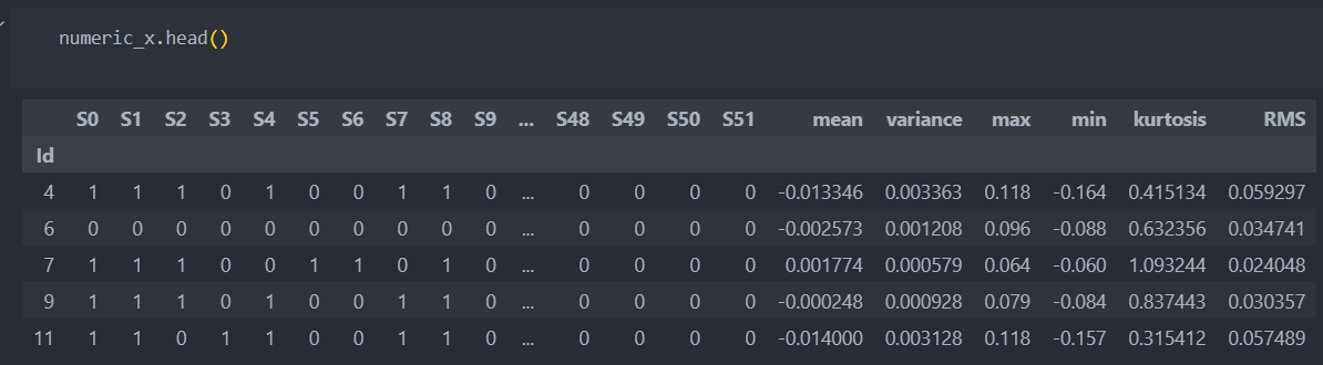

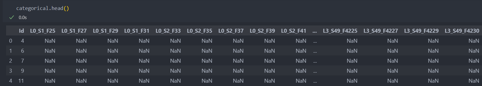
범주형 데이터

'Id'를 index로 설정하고 진행하도록 한다.

df = categorical.copy()

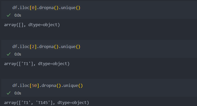
df.set_index('Id', inplace=True)

Id별 결측치가 아닌 값 확인

범주형 데이터는 수치형 데이터보다 결측값이 더 많다.
Id(행)별로 어떤 값들이 있는지 확인해보자.

모든 데이터가 결측인 Id(행)도 존재하기에 모든 행을 탐색하며 등장한 값을 확인해본다.
코드는 'T'로 시작하는 어떤 값이다.

모든 Id(행)을 탐색하며 결측이 아닌 값이 등장할 때의 모든 code 값들을 codes로 저장한다.

codes = []

for idx, row in df.iterrows():
    for code in row.dropna().unique():
        if code not in codes:
            codes.append(code)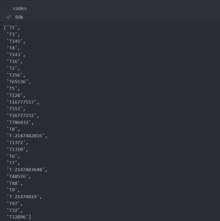

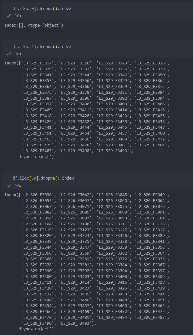
T 코드가 등장한 스테이션 확인

코드가 등장한 공정을 확인해보자.

아래와 같이 코드가 등장하지 않았다면 모든 값이 결측일 것이고,
코드가 등장한 공정은 아래와 같이 모든 공정에서 나타나는 것이 아닌 특정 공정에서만 진행되었음을 확인할 수 있다.

수치형 데이터에서와 같이, 범주형 데이터도 '스테이션'을 기준으로 데이터를 정리하기 위해서,
코드가 등장한 스테이션을 기준으로 정리하도록 한다.
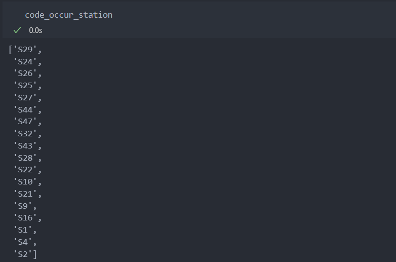
그래서 코드가 등장한 스테이션을 정리한다.

code_occur_station = []

for idx, row in df.iterrows():
    for col in row.dropna().index:
        if col.split('_')[1] not in code_occur_station:
            code_occur_station.append(col.split('_')[1])

아래와 같이 코드가 등장한 스테이션을 확인할 수 있다.
모든 스테이션에서 코드가 등장하는 것은 아님을 알 수 있다.

Id별 등장한 코드와 스테이션 정리

탐색한 코드와 스테이션을 조합하여, 코드가 스테이션에 등장하였으면 1을 아니면 0을 부여하는 작업을 진행한다.
ex) '스테이션_코드'

스테이션과 코드를 itertools의 product를 사용하여 조합한 컬럼을 생성하고,
모든 Id(행)별로 해당 스테이션에 코드가 등장하였다면 1을 아니면 0으로 데이터를 생성한다.

코드가 등장한 공정별로

스테이션이 등장한 경우와

코드가 등장 경우를

확인하여 'and' 조건으로 묶어서 데이터를 생성한다.

먼저 '스테이션 + 코드' 컬럼을 생성한다.

code_x_columns = []

for station, code in itertools.product(code_occur_station, codes):
    code_x_columns.append(station + ' ' + code)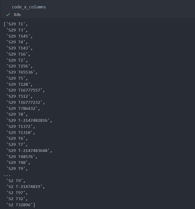

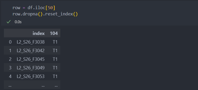
그리고 모든 행을 iterrows()로 순회하며, 해당 행에 코드가 등장했었던 스테이션과 코드를 조합하여
행별로 True/False로 저장한 후 int화 하여 1과 0으로 데이터를 생성한다.

# 모든 Id(행)별 등장한 코드와 스테이션을 탐색하기에 시간이 오래 걸린다.
code_x = []

for idx, row in df.iterrows():
    if sum(row.notnull()) == 0: # 모든 컬럼이 결측치인 경우
        record = [0] * len(code_occur_station) * len(codes) # 스테이션과 코드의 조합 가짓수 길이를 0으로
    
    else: # 컬럼 중 코드 값이 있는 경우
        record = []
        
        for station, code in itertools.product(code_occur_station, codes): # 스테이션과 코드의 조합
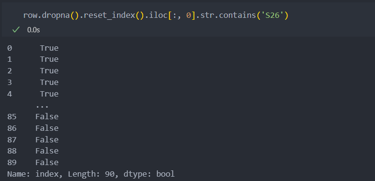
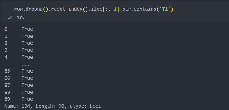
            drop_row = row.dropna().reset_index()
            condition = (drop_row.iloc[:, 0].str.contains(station)) & (drop_row.iloc[:, 1].str.contains(code))
            record.append(sum(condition) > 0) # True/False
    
    code_x.append(record)

code_x = pd.DataFrame(code_x, columns=code_x_columns, index=df.index)
code_x = code_x.astype(int)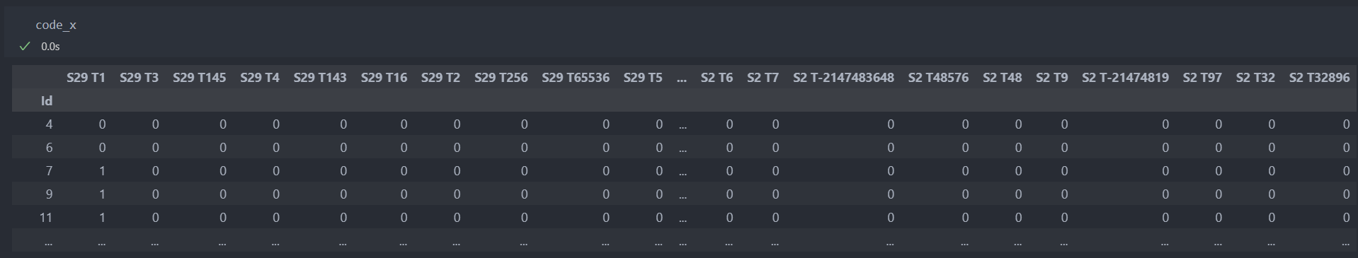

모든 행을 순회하며 각 스테이션과 코드의 조합도 살펴보기 때문에 시간이 오래 걸린다.
그래서 수치형 데이터를 정리한 것과 범주형 데이터를 정리한 것을 merge하여 미리 저장하고,
다음부터 저장된 데이터를 불러와서 모델링을 진행한다.

데이터 저장

# 데이터 merge
X = pd.merge(numeric_x, code_x, left_index=True, right_index=True)

# 데이터 저장
X.to_csv('./data/data_x.csv')

모델링

특징(컬럼) 대부분이 이진형 데이터이며, 샘플과 특징이 모두 많은 편이므로 서포트 백터 머신 모델을 사용한다.
그리고 클래스 불균형이 존재하므로 class_weight를 조정하기로 한다.
평가지표는 f1_score를 사용한다.

from sklearn.svm import SVC
from sklearn.metrics import f1_score
from sklearn.model_selection import train_test_split, ParameterGrid
from sklearn.preprocessing import MinMaxScaler
from sklearn.feature_selection import *

학습

학습/평가 데이터 분리

train_x, test_x, train_y, test_y = train_test_split(X, Y, stratify=Y)

스캐일링

MinMax 스케일링을 진행한다.

scaler = MinMaxScaler().fit(train_x)

train_x = pd.DataFrame(scaler.transform(train_x), columns=train_x.columns, index=train_x.index)
test_x = pd.DataFrame(scaler.transform(test_x), columns=test_x.columns, index=test_x.index)

하이퍼 파라미터 설정

파라미터 설정 시 class_weight를 조정한다.

서포트 백터 머신(SVM)에 적용되는 커널은 대부분 기저함수로 변환하였을 때 무한대의 차원을 가지기에 비선형성을 처리할 수 있다.
서포트 백터 머신의 대표 커널인 linear(선형) 커널과 RBF(가우시안) 커널의 경우로 나눠서 사용하기로 한다.
그리고 하이퍼 파라미터의 수가 많기에 조절하면서 진행하도록 한다.

# CI = 클래스 불균형 비율
CI = train_y.value_counts().iloc[0] / train_y.value_counts().iloc[-1]
CI > 186.5

# linear 커널
param_grid_linear = ParameterGrid({
                                    'C':[10**-2, 10**-1, 10**0, 10**1, 10**2],
                                    'class_weight':[{0:1, 1:CI * w} for w in np.arange(0.1, 1.1, 0.2)],
                                    'kernel':['linear'],
                                    'random_state':[29, 1000]
})
# 가우시안 커널
param_grid_rbf = ParameterGrid({
                                    'C':[10**-2, 10**-1, 10**0, 10**1, 10**2],
                                    'class_weight':[{0:1, 1:CI * w} for w in np.arange(0.1, 1.1, 0.2)],
                                    'kernel':['rbf'],
                                    'random_state':[29, 1000],
                                    'gamma':[10**-2, 10**-1, 10**0, 10**1, 10**2]
})

학습 진행

best_score = -1
iter_num = 0

for k in range(150, 10, -10):
    print(k)
    selector = SelectKBest(mutual_info_classif, k=k).fit(train_x, train_y)
    selected_features = train_x.columns[selector.get_support()]

    for grid in [param_grid_linear, param_grid_rbf]:
        for param in grid:
            model = SVC(**param).fit(train_x[selected_features], train_y)
            pred = model.predict(test_x[selected_features])
            score = f1_score(test_y, pred)

            if score > best_score:
                best_score = score
                best_mode = model
                best_features = selected_features
            
            iter_num += 1
            print(f'{iter_num}/{max_iter} best score : {best_score}')

적용

평가 지표 f1 score가 가장 높았던 파라미터와 features로 최종 모델을 선정하여 test 진행

pipeline 함수

데이터 전처리를 거쳐왔던 모든 전처리를 함수로 만들어 데이터 예측 진행

def pipeline(numeric_df, categorical_df,
             total_stations, remove_outliers, extract_statistical_feature,
             codes, code_occur_station, 
             scaler, model, features):
    # 데이터 카피
    numeric_df_copy = numeric_df.copy()
    categorical_df_copy = categorical_df.copy()
    
    ## 수치형 데이터 정제
    numeric_df_copy.set_index('Id', inplace = True)
    
    # station_X 생성
    station_X = []
    
    for ind, row in numeric_df_copy.iterrows():
        if sum(row.notnull()) == 0:
            station_X.append(np.zeros(len(total_stations))) # whole stations에 포함된 stations를 추가 
        else:
            not_null_columns = numeric_df_copy.columns[row.notnull()]
            stations = pd.Series(not_null_columns).str.split('_', expand = True).iloc[:, 1].drop_duplicates().tolist()

            station_X.append(np.isin(total_stations, stations)) # whole stations에 포함된 stations를 추가 

    station_X = pd.DataFrame(station_X, index = numeric_df_copy.index, columns = total_stations)
    station_X = station_X.astype(int)
    
    # stat_feature_X 생성
    stat_feature_X = numeric_df_copy.apply(extract_statistical_feature, axis = 1)
    stat_feature_X.rename({0:"mean", 1: "variance", 2:"max", 3:"min", 4:"kurtosis", 5:"RMS"}, axis = 1, inplace = True)
    
    numeric_X = pd.merge(station_X, stat_feature_X, left_index = True, right_index = True)
    
    ## 범주형 데이터 정제
    categorical_df_copy.set_index('Id', inplace = True)
    
    # code_X_columns 생성
    code_X_columns = []
    for station, code in itertools.product(code_occur_station, codes):
        code_X_columns.append(station + "_" + code)
    
    # code_X 생성
    code_X = []
    for ind, row in categorical_df_copy.iterrows():
        if sum(row.notnull()) == 0: # 전부 결측이면 굳이 아래 for문을 순회할 필요가 없음
            record = [0] * len(code_occur_station) * len(codes)

        else:
            record = []
            for station, code in itertools.product(code_occur_station, codes):
                dropna_row = row.dropna().reset_index()
                cond = (dropna_row.iloc[:, 0].str.contains(station)) & (dropna_row.iloc[:, 1].str.contains(code))
                record.append(sum(cond) > 0) # True, False로 값을 넣음
        code_X.append(record)
    
    code_X = pd.DataFrame(code_X, columns = code_X_columns, index = categorical_df_copy.index)
    code_X = code_X.astype(int)
    
    # X 생성
    X = pd.merge(numeric_X, code_X, left_index = True, right_index = True)
    
    # 스케일링
    X = pd.DataFrame(scaler.transform(X), columns = X.columns, index = X.index)
    
    # 특징 선택
    X = X[features]
    
    # 모델 예측
    output = model.predict(X)
    
    return output

적용

# test data
numeric_test_df = pd.read_csv('./data/test_numeric.csv')
categorical_test_df = pd.read_csv('./data/test_categorical.csv')

# pipeline 적용하여 예측
pipeline(numeric_test_df, categorical_test_df,
             total_stations, remove_outliers, extract_statistical_feature,
             codes, code_occur_station, 
             scaler, best_model, best_feature)

기대 효과

불량 제품을 예측하여 저렴한 비용으로 품질 좋은 제품 제공 및 Bosch사의 이미지 개선