Pytorch를 간단히 다루어본 적이 있는데, 앞으로의 연구에 익숙하게 활용하기 위해 Pytorch 내용을 정리해보려 한다.
대부분의 내용은 유튜브의 '모두를 위한 딥러닝 시즌2'를 참고하였다.
기본적인 딥러닝 내용은 어느 정도 알고 있다고 가정하고, PyTorch 실습 내용 위주로 정리해두었다.
간단한 설명이 포함된 실습 자료는 다음 Github를 참조하자.
1. Logistic Regression 개요
앞서 살펴봤던 Linear Regression은 수로 표현하는 설명변수와 연속형 숫자로 이루어진 종속변수의 관계를 선형으로 어떻게 잘 나타낼 수 있는지를 살펴보기 위한 것이었다.
이에 반해 Logistic Regression의 경우, Classification 문제에 자주 사용되는데, 이때에는 종속변수 가 연속형 숫자가 아닌 범주(Class)를 나타낸다.
1) Binary Classification
먼저 종속변수가 두 개인, 즉 데이터가 두 가지로 나뉘는 경우를 생각해보자. 이를 Binary Classification 문제라 한다.
Hypothesis로는 다음과 같은 sigmoid 함수가 많이 사용된다. sigmoid 함수는 0과 1 사이의 값을 출력해주므로, 이는 확률과 비슷한 개념으로 볼 수 있다.
또한 Cost로는 다음과 같은 Binary Cross-entropy가 많이 사용된다.
그리고 파라미터의 업데이트는 앞선 방법과 동일하게 Gradient Descent로 진행된다.
Implementation
먼저 다음과 같이 import를 진행한다.
import torch
import torch.nn as nn
import torch.nn.functional as F
import torch.optim as optim
그리고 다음 코드를 통해 seed를 부여해서 같은 코드에 대해 추후에 같은 결과를 제공해줄 수 있다.
# For reproducibility (나중에도 같은 결과 제공 - seed 부여)
torch.manual_seed(1)
Training Data
다음과 같은 x_train, y_train 데이터를 가정하자.
x_data = [[1, 2], [2, 3], [3, 1], [4, 3], [5, 3], [6, 2]] # 6 by 2
y_data = [[0], [0], [0], [1], [1], [1]] # 6 by 1

x_train = torch.FloatTensor(x_data)
y_train = torch.FloatTensor(y_data)
Computing the Hypothesis
PyTorch에서 제공하는 'torch.exp()'함수를 통해 exponential function을 쉽게 구현할 수 있다.
W = torch.zeros((2, 1), requires_grad=True)
b = torch.zeros(1, requires_grad=True)

hypothesis = 1 / (1 + torch.exp(-(x_train.matmul(W) + b)))
또는 간단히 'torch.sigmoid()'함수를 사용할 수도 있다.
hypothesis = torch.sigmoid(x_train.matmul(W) + bComputing the Cost Function
cost 수식을 구현하기 위해, 다음과 같이 구현한다.
losses = -(y_train * torch.log(hypothesis) +
            (1 - y_train) * torch.log(1 - hypothesis))
cost = losses.mean()
또는 PyTorch의 'F.binary_cross_entropy()'함수를 사용할 수도 있다.
F.binary_cross_entropy(hypothesis, y_train)Whole Training Procedure
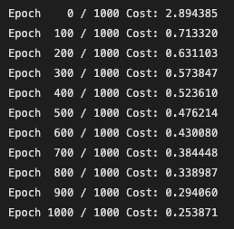
전체적으로 학습 과정과 그 결과를 살펴보자.
# 모델 초기화
W = torch.zeros((2, 1), requires_grad=True)
b = torch.zeros(1, requires_grad=True)

# optimizer 설정
optimizer = optim.SGD([W, b], lr=1) # SGD 사용

nb_epochs = 1000
for epoch in range(nb_epochs + 1):
    # Cost 계산
    hypothesis = torch.sigmoid(x_train.matmul(W) + b)
    cost = F.binary_cross_entropy(hypothesis, y_train)

    # cost로 H(x) 개선
    optimizer.zero_grad()
    cost.backward()
    optimizer.step()

    # 100번 마다 로그 출력
    if epoch % 100 == 0:
        print('Epoch {:4d} / {} Cost: {:.6f}'.format(
            epoch, nb_epochs, cost.item()
        ))
Evaluation
모델을 학습한 이후에는 모델이 test set에 얼마나 잘 작동하는지 (일반화 성능이 얼마나 좋은지가 인공지능 모델의 최종 목표) 알아보아야 한다.
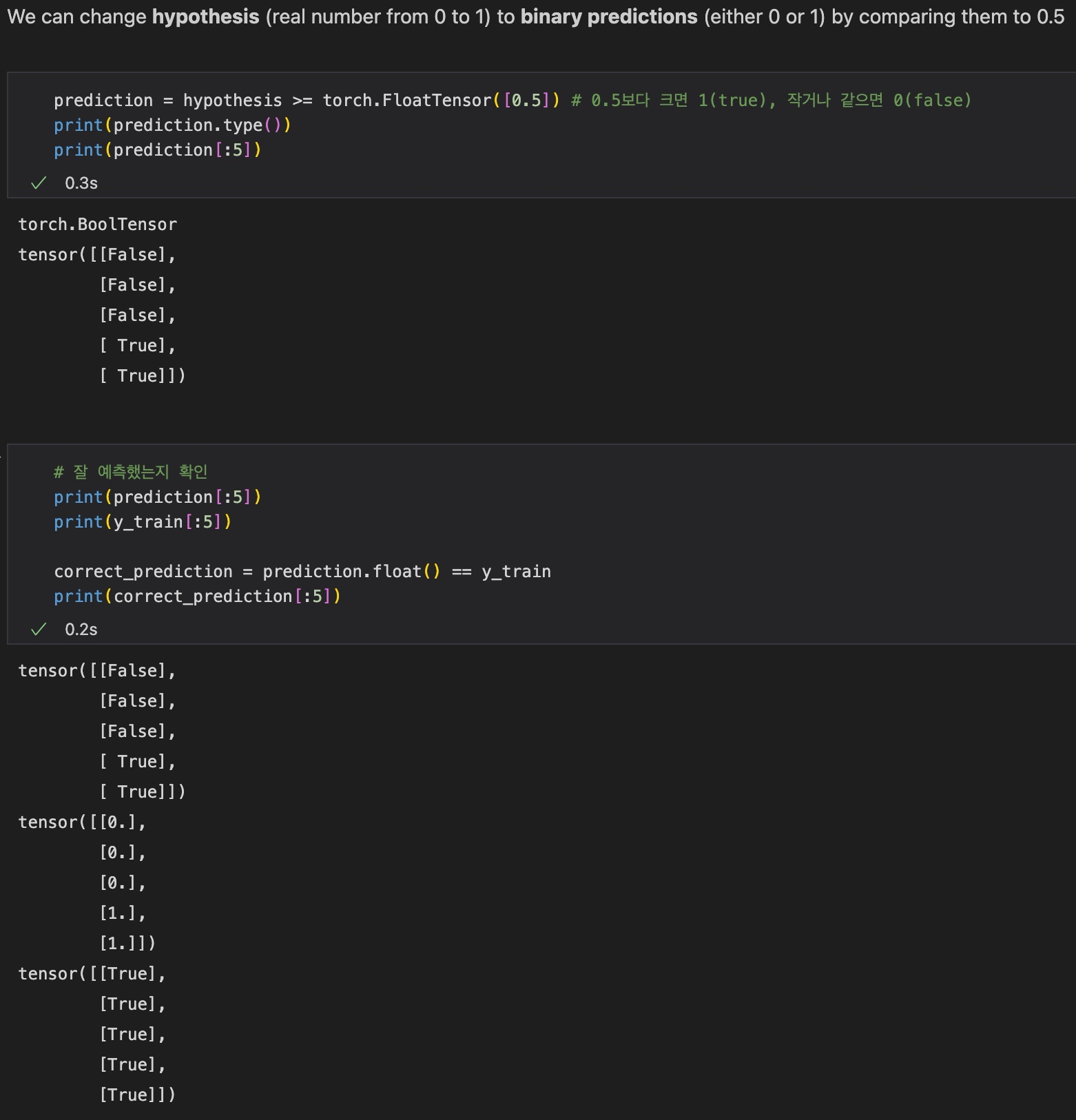
hypothesis = torch.sigmoid(x_test.matmul(W) + b)
prediction = hypothesis >= torch.FloatTensor([0.5])
correct_prediction = prediction.float() == y_train
hypothesis는 0과 1사이의 실수 값이므로, 그 값이 0.5보다 크면 1, 같거나 작으면 0을 할당하여 false(0) 또는 true(1)의 값을 갖는 binary prediction으로 변경해준다.
이때 prediction의 datatype은 BoolTensor이다.
다음으로 correct_prediction을 출력하여 예측을 제대로 했는지 살펴본다. 최종 결과는 다음과 같다.
Higher Implementation with Class
앞서 Linear Regression에서도 그랬듯이, Class를 활용하여 효율적인 코드를 작성할 수 있다.
class BinaryClassifier(nn.Module):
def __init__(self):
super().__init__()
self.linear = nn.Linear(2, 1) # 2개 입력받을 것
self.sigmoid = nn.Sigmoid()
def forward(self, x):
return self.sigmoid(self.linear(x))
model = BinaryClassifier()
# optimizer 설정
optimizer = optim.SGD(model.parameters(), lr=1)
nb_epochs = 100
for epoch in range(nb_epochs + 1):
# H(x) 계산
hypothesis = model(x_train)
cost = F.binary_cross_entropy(hypothesis, y_train)
# cost로 H(x) 계산
optimizer.zero_grad()
cost.backward()
optimizer.step()
# 20번마다 로그 출력
if epoch % 20 == 0:
prediction = hypothesis >= torch.FloatTensor([0.5])
correct_prediction = prediction.float() == y_train
accuracy = correct_prediction.sum().item() / len(correct_prediction)
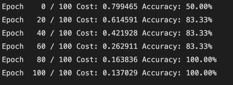
print('Epoch {:4d} / {} Cost: {:.6f} Accuracy: {:2.2f}%'.format(
epoch, nb_epochs, cost.item(), accuracy * 100,
))결과는 아래와 같다.
2. Softmax Classification
앞서 종속변수가 두 가지 범주인 경우를 살펴보았다.
하지만, 실생활에서는 3개 이상의 클래스를 가지는 경우가 훨씬 많다.
이때 Softmax fuction을 사용한다.
1) Softmax Function
Softmax Function은 다음 수식을 통해 (특히 3개 이상의) 클래스들 중 특정 클래스에 속할 확률을 계산해준다.
각 softmax 값을 모두 더하면 1이 되므로 확률의 개념이라고 생각할 수 있다.
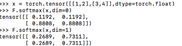
예를 들어, 다음과 같은 tensor가 있다고 가정하자.
x = torch.tensor([[1, 2], [3, 4]])이때, PyTorch에서 제공하는 'softmax' 함수를 사용하면 간단하게 softmax를 계산할 수 있다.
단, dimension에 유의해야 한다. dim이라는 인자를 입력해주고, 해당하는 축을 기준으로 normalize를 한다. 즉, 위의 예시에서 dim=0인 경우 열의 합이 1, dim=1인 경우 행의 합이 1이 된다.
2) Cross Entropy Loss (Low-level)
이제 Multi-class classification 분제에서 cross entropy를 구해보자.
이때 는 예측값(확률), 는 정답값(확률)이다.
다음 예시 코드를 보자.
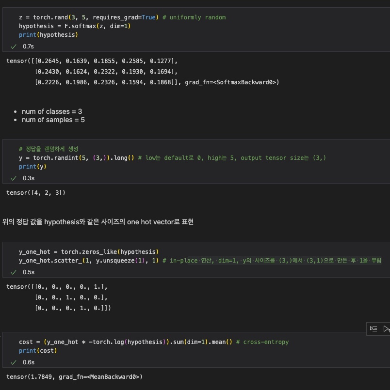
z = torch.rand(3, 5, requires_grad=True) # uniformly random
hypothesis = F.softmax(z, dim=1)
print(hypothesis)

# 정답을 랜덤하게 생성
y = torch.randint(5, (3,)).long() # low는 default로 0, high는 5, output tensor size는 (3,)
print(y)
3 × 5 크기의 tensor를 생성하고, softmax 함수를 적용한다. 이떄 class는 3개, sample은 5개이다.
이에 따라 3개의 클래스를 갖는 정답 y를 생성한다.
예를 들어 tensor([4, 2, 3])이라는 y가 생성되었다고 생각하자. 이것을 바로 사용할 수는 없으니, 각 값에 대해 해당 index만 1이고 나머지 index는 0인 one hot vector로 정답을 바꾸어준다.
y_one_hot = torch.zeros_like(hypothesis)
y_one_hot.scatter_(1, y.unsqueeze(1), 1) # in-place 연산
# dim=1, y의 사이즈를 (3,)에서 (3,1)으로 만든 후 1을 뿌림

cost = (y_one_hot * -torch.log(hypothesis)).sum(dim=1).mean() # cross-entropy
print(cost)
그 후, cross-entropy로 cost를 계산한다.
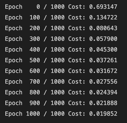
전체 결과는 다음과 같다.
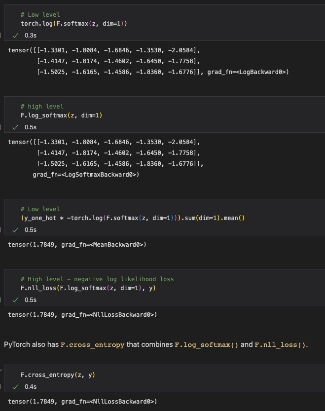
하지만 위와 같이 복잡한 과정을 'F.cross_entropy'라는 함수로 쉽게 대체할 수 있다.
사실 'F.cross_entropy' 함수도 softmax 함수 결과에 로그를 바로 씌워주는 'F.log_softmax()'함수와 Negative Log Likelihood Loss를 계산하는 'F.nll_loss()'함수의 기능을 합한 것으로, 위와 같은 로직을 갖는다.
Implementation
1) Training with F.cross_entropy
전체 Training 과정은 다음과 같다.
x_train = [[1, 2, 1, 1],
[2, 1, 3, 2],
[3, 1, 3, 4],
[4, 1, 5, 5],
[1, 7, 5, 5],
[1, 2, 5, 6],
[1, 6, 6, 6],
[1, 7, 7, 7]] # 8 samples, 4 input vectors(dim)
y_train = [2, 2, 2, 1, 1, 1, 0, 0] # 3 classes
x_train = torch.FloatTensor(x_train)
y_train = torch.LongTensor(y_train) # discrete
# 모델 초기화
W = torch.zeros((4, 3), requires_grad=True)
b = torch.zeros(1, requires_grad=True)
# optimizer 설정
optimizer = optim.SGD([W, b], lr=0.1)
nb_epochs = 1000
for epoch in range(nb_epochs + 1):
# Cost 계산 (직접 구현)
# hypothesis = F.softmax(x_train.matmul(W) + b, dim=1)
# y_one_hot = torch.zeros_like(hypothesis)
# y_one_hot.scatter_(1, y_train.unsqueeze(1), 1)
# cost = (y_one_hot * -torch.log(F.softmax(hypothesis, dim=1))).sum(dim=1).mean()
# Cost 계산 (cross_entropy 함수로 구현)
z = x_train.matmul(W) + b
cost = F.cross_entropy(z, y_train)
# cost로 H(x) 개선
optimizer.zero_grad()
cost.backward()
optimizer.step()
# 100번마다 로그 출력
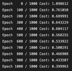
if epoch % 100 == 0:
print('Epoch {:4d} / {} Cost: {:.6f}'.format(
epoch, nb_epochs, cost.item()
))
2) High-level Implementation with nn.Module
이제 Class를 이용한 High-level 구현을 살펴보자.
모두 배운 내용이니 코드를 보면 금방 이해할 수 있을 것이다.
class SoftmaxClassifierModel(nn.Module):
    def __init__(self):
        super().__init__()
        self.linear = nn.Linear(4, 3) # num of output classes = 3

    def forward(self, x):
        return self.linear(x)

model = SoftmaxClassifierModel()

# optimizer 설정
optimizer = optim.SGD(model.parameters(), lr=0.1)

nb_epochs = 1000
for epoch in range(nb_epochs + 1):
    # Cost 계산
    # hypothesis = F.softmax(x_train.matmul(W) + b, dim=1)
    # y_one_hot = torch.zeros_like(hypothesis)
    # y_one_hot.scatter_(1, y_train.unsqueeze(1), 1)
    # cost = (y_one_hot * -torch.log(F.softmax(hypothesis, dim=1))).sum(dim=1).mean()
    # z = x_train.matmul(W) + b
    # cost = F.cross_entropy(z, y_train)

    # H(x) 계산
    prediction = model(x_train)

    # Cost 계산
    cost = F.cross_entropy(prediction, y_train)

    # cost로 H(x) 개선
    optimizer.zero_grad()
    cost.backward()
    optimizer.step()

    # 100번마다 로그 출력
    if epoch % 100 == 0:
        print('Epoch {:4d} / {} Cost: {:.6f}'.format(
            epoch, nb_epochs, cost.item()
        ))