"Context Encoders: Feature Learning by Inpainting” 논문을 리뷰해보는 시간을 갖겠습니다.
Abstract
context-based pixel 예측을 통해 unsupervised visual feature learning algorithm을 제시.
Context Encoder라는 이름의 모델이고, 임의의 Image의 어떤 region을 주변 context를 이용해 예측, 생성하는 convolution neural network.
위 task를 수행하기 위해서는, 모델이 두 가지 역할을 수행해야함.
-
전체 이미지의 content에 대한 이해.
-
missing part(region)에 대한 그럴듯한 예측
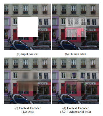
context encoder를 학습 시킬 때, reconstruction loss만을 사용한 것과 adversarial loss를 함께 사용한 것을 비교 실험을 했고, 후자가 더 좋은 성능을 보였음.
또한 context encoder가 단지 appearance만 학습하는 것이 아니라, 어떤 시각적 구조의 의미까지 학습을 하는 것을 확인할 수 있었음.
classification, detection, segmentation task를 위한 CNN을 이런 context encoder의 feature learning 특징을 이용해pre-training 하고 양적 평가도 진행했음.
또한 context encoder는 semantic inpainting task에 여러 방법으로 사용될 수 있음.
Introduction
위 사진을 보면 우리 인간은 사진의 빈 공간을 머릿속에서 채워넣거나, 혹은 실제로 그려넣을 수도 있음.
이는 실제 세상의 이미지가 매우 다양하긴 하지만, highly structured 되어 있고, 인간은 그 structure에 대해 깊은 이해가 있기 때문.
논문에서는 이런 structure를 잘 이해하고 또 예측할 수 있는 Convolution neral networks를 학습시킬 수 있음을 제시.
missing region이 존재하는 이미지에 대해 그 region을 regression 할 수 있는 network를 학습시켰는데, context encoder라고 명명함.
context encoder는 이미지의 context를 latent feature representation로 compact 시키는 encoder와 그 feature representation을 이용해 missing region을 생성하는 decoder로 이루어져 있음.
context encoder는 Autoencoder와 비슷한 구조를 갖고 있는 만큼 밀접한 관계를 갖고 있음.
Autoencoder는 input image를 받아 low dimensional bottleneck layer를 통과시켜 이미지에 대해 feature representation 얻지만, 이런 방법은 Semantic meaningful representation을 얻기보다는 Image content를 압축시킴에 더 강한 의미가 있음.
Denoising autoencoder는 이런 문제를 input image에 약한 noise를 추가함으로써 이를 해결했는데, 하지만 이런 약한 noise는 그렇게 효과적이지 못함.
context encoder는 더 어려운 task를 해결해야 함.
- 주변 픽셀로부터 어떤 hint도 얻지 못한 상황에서, large missing area를 채우는 task
이런 task는 scene에 대해 더 깊은 semantic understanding, large spatial extents에 대해 high-level feature을 synthesize 할 수 있어야 함.
Autoencoder과 동일하게 context encoder는 unsupervised learning 이용.
두 가지 loss function을 이용했는데
-
Reconstruction(L2) loss : missing region의 structure를 이미지 전체 context와 관련있게 capture 할 수 있도록 해줌.
-
Adversarial loss : missing region을 채울 수 있는 여러 후보군의 distribution 중 더 좋은 선택을 할 수 있게 해줌.
encoder와 decoder 각각 독립적으로 평가를 진행했음.
encoder의 경우 context of image를 encoding 하는 것과 그 결과로 나온 feature를 이용해 original과 semantically similar 한 patch를 만드는 것을 확인했음.
이런 feature의 quality를 측정하기 위해 fine-tuning encoder를 여러가지 task에 적용해봤고, 이는 현재 State of the art method들에게도 밀리지 않는 모습을 보였음.
decoder의 경우, hole filling과 같은 task에서 realistic image와 매우 유사한 수준의 task 수행 능력을 보였음.
Context encoders for image generation
context encoder에 대한 설명.
Encoder-decoder pipeline
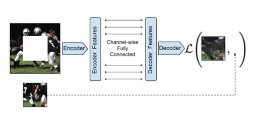
context encoder의 전체적인 구조(위 사진)는 encoder decoder pipeline.
encoder는 missing region이 존재하는 image를 input으로 받아 image의 laten feature representation을 생성
decoder는 이 feature representation을 받아 이용하여 image의 missing region을 채워넣음.
중요한 점은 encoder와 decoder를 연결할 때, channel-wise fully connected layer를 이용해 연결을 해야한다는 것.
이런 연결 방법은 decoder의 unit들이 전체 image content에 대해 추론할 수 있게 함.
Encoder
encoder는 AlexNet architecture에서 유래했음.
227 x 227 size의 image를 input으로 받으면, 처음 5개의 convolution layer + pooling layer들을 이용해 6 x 6 x 256 크기의 feature representation을 계산.
AlexNet과 다른점은 context encoder의 경우 ImageNet classification을 위해 학습이 되지 않았다는 것(pre-trained 되지 않았다는 의미), 더 나아가 context encoder는 context prediction을 위해 from scratch로 randomly initialized weights을 이용해 학습했음.
하지만, encoder의 구조를 convolution layer만 사용해 만든다면 feature map의 특정 corner에 대한 정보를 다른 corner에 전달할 수가 없음.
이런 문제점들을 현재 방법론으로는 fully connected layer를 통해 해결하고 있음.
context encoder의 latent feature의 dimension = 6 x 6 x 256 = 9216임.
이걸 fully connected layer로 연결하면 parameter수가 말도 안되게 증가할 것.
따라서 encoder와 decoder를 연결하는 부분에 우리는 channel wise fully connected layer를 이용
Channel-wise fully-connected layer
이 layer는 각 feature map을 activation function에 통과시킴으로써 information을 전달.
input : m개의 n x n feature map
output: m개의 n x n feature map
fully connected layer와 다른 점은 fully connected layer는 각각의 feature map을 연결해주는 parameter가 존재하지만, channel-wise의 경우 각 feature map에 대해 독립적으로 information 전달.
그러므로
fully connected 의 parameter 수 :
channel wise의 parameter 수 :
Decoder
channel-wise FC layer를 통해 전달받은 feature는 5개의 up-convolution layer를 통과(각각 ReLU 함수 함께 존재).
up-convolution과 non-linearity(ReLU)는 non-linearity weighted upsampling을 일으키며 원 해상도의 이미지를 생성.
Loss function
context encoder는 missing region의 ground truth를 regression 하도록 train 됨.
Reconstruction(L2) loss와 Adversarial loss를 이용해 학습을 시켰음.
Reconstruction loss는 전체적인 구조에 알맞게 missing region에 대한 구조를 만들 수 있도록 영향을 미침.
Adversarial loss의 경우 예측값(missing region에 대한 regression값)이 실제와 비슷하도록 영향을 미침
input image =
context encoder 가 만드는 output =
binary mask(missing region에 대하여 1, 그 외의 값은 0을 가지는 이미지) =
로 놓자(binary mask는 training 과정에 자동적으로 생성됨.)
Reconstruction Loss
= ( - ((1 - ) ))
= element-wise product
L1, L2 loss 두 가지 모두 실험했으나, 둘 사이에 큰 차이가 없는 것을 확인할 수 있었음.
reconstruction loss가 predicted object(ex: missing region)에 대해 대략적인 outline을 decoder가 만들 수 있도록 하지만, high frequency detail에 대해서는 종종 실패하는 모습을 보임.
이는 L2(or L1) loss가 종종 highly accurate texture 보다 blurry solution을 선택할 때 발생되는 현상.
이런 현상은 loss가 blurry solution이 더 안전하다고 생각했기 때문임.
즉 pixel-wise에서 평균값으로는 최적의 loss값을 내는 solution을 선택할 때, 그 solution이 blurry solution이라는 뜻.
이 문제는 후술할 Adversarial loss로 해결.
Adversarial Loss
Adversarial loss는 Generative Adversarial Networks(GAN)에서 유래했음.
GAN에서는, Generative model 가 data distribution을 학습시키기 위해 adversarial discriminative model 를 함께 학습시키며 generative model을 위한 loss gradients를 제공함.
와 는 모두 parametric function(ex: deep networks)임.
GAN에 대해서 요약하자면 는 최대한 '진짜'(real data)같은 sample을 만들어 가 그 sample 에 대해 '진짜'라고 판단하도록 헷갈리게 생산하고, 는 그걸 잘 구별해내도록 학습하는 것임.
우리는 context encoder를 GAN의 generator에 대입하면서 위 framework를 적용시켰음.
우리의 adversarial loss는 다음과 같음.
= +
Joint Loss
우리가 사용하는 loss를 총 정리하자면
= +
Adversarial Loss는 AlexNet 구조를 이용한 inpainting task를 할 때만 수행하고 있음.
Region masks
context encoder의 input image는 한 곳 이상의 missing region이 존재함.
그런 missing region은 여러 형태로 나타날 수 있고 이에 대해 우리는 세 가지 종류로 정리했음.
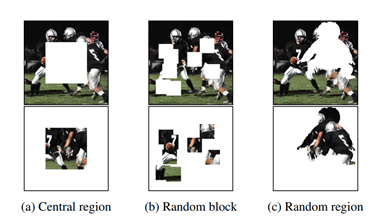
위 사진은 그 종류를 나타낸 것임.
Central region
가장 간단한 형태인 가운데에 정사각형 모양의 missing region이 존재하는 경우.
inpainting이 잘 되긴 하지만, network가 학습하는 low level image feature는 이미지의 중앙 부분에 latching 되는 경향이 있음.
그런 low level feature는 missing region이 없는 image에 잘 일반화되어 있지는 않음.
Random block
missing region에 대해 생성하는 image feature가 latching 하는 경향을 막기 위해, missing region을 random하게 생성했음.
하나의 큰 missing region을 만드는 대신에, 이미지 여러 부분에서 missing region을 만들었음(이미지의 1/4 가량).
하지만 여전히 latching 하는 경향이 있음.
Random region
따라서 이미지에서 임의로 추출한 모양으로 missing region을 생성했는데, 이때 추출한 모양은 PASCAL VOC 2012 dataset을 기반으로 했음.
이때 임의로 추출한 모양은 이미지에서 어떤 의미도 갖고 있지 않고(ex:위 사진의 (c)에서 missing region을 보면 해당 region이 이미지에서 어떤 의미(미식 축구 선수, 잔디)를 갖고 있지 않은 무작위적인 image patch) 연관관계도 없음.
이 방법대로 실험한 결과 모델이 좀 더 general한 feature를 학습 및 생성함을 확인했고, 이후 모든 실험은 Random region을 기반으로 수행했음.
Implementation details
모든 pipeline은 caffe와 torch를 이용했음.
optimization의 경우 ADAM을 이용했음.
input image의 missing region의 경우 constant mean value로 채워넣음.
Pool-free encoders
모든 pooling layer를 같은 kernel size와 stride를 갖고 있는 convolution layer로 대체했음.
전체적인 stride는 같지만 inpainting 결과가 좀 더 좋았음.
직관적으로 생각했을 때, reconstruction 과정에서 pooling을 쓸 이유가 없었음.
classification을 수행한다고 가정해보자.
이럴 경우 pooling은 spatial invariance(공간 특성을 불변시킴)의 이점이 있지만, 우리가 행하는 reconstruction task에서는 효과가 없음.
이전 work들과 일관성을 갖기 위해, 우리는 feature learning results를 구함에 있어서 Alexnet 구조(with pooling)를 그대로 사용했음.
Evaluation
encoder 평가는 encoder가 생성하는 feature의 semanctic quality와 transferbility를 평가했음.
ParisStreetView dataset과 ImageNet dataset을 label 없이 이용했음.
evaluation은 두 가지 측면으로 나눌 수 있는데, 첫번째로는 context encoder의 semantic inpainting 능력을 측정했고, 두번째로는 encoder가 학습한 feature를 다른 task(classification, detection, semantic segmentation)에 이용해본 결과를 측정했음.
실험 결과는 이전 unsupervised, self-supervised들과 비교했음.
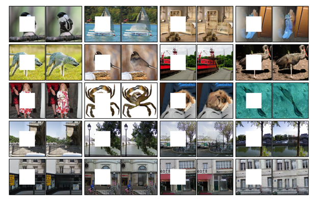
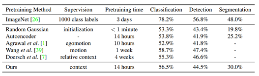
사진은 차례대로 semantic inpainting 결과와 context encoder가 학습한 feature를 이용해 다른 task(classification, detection, segmentation) 을 수행한 결과임.
좋은 inpainting 수행 능력과 짧은 pretraining time으로도 다른 method들(Random Gaussian, Autoencoder 등)에 비해 좋은 task 수행 능력(classification, detection, segmentation)을 보여줬음.
Conclusion
context encoder는 semantic inpainting task에서 state of the art(SOTA)를 향상시켜줬고, context encoder가 학습하는 feature 또한 여러 방면에서 쓰일 수 있음을 보였음.