
✔ Classification
개요
- 자동으로 어떤 결정을 해야 하는 종류의 문제를 접했을 때, 결정해야 할 Target이 범주형인 경우, 예측 모형은 새로운 자료에 대한 분류가 주목적이 되며, 결과가 이미 나와 있는 경우이므로 지도학습이다.
유형
- 이진 분류(둘 중 하나) 와 다중 분류(카테고리 중 하나)
- 선형 분류 와 비선형 분류
- 다중 분류는 여러 개의 이진 분류 문제로 돌려서 해결하는 것도 가능합니다.
sklearn에서 예측 함수
- predict
- 클래스를 반환 - predict_proba
- 각 클래스에 대한 확률을 반환
- 확률을 가지고 Cut Off(절사)를 통해서 경향 점수로부터 결정을 내림
접근 방식
- 어떤 record가 속할 것이라고 예쌍되는 관심 클래스에 대한 Cut OFf proba를 설정
- record가 관심 클래스에 속할 확률을 추정
- 확률이 Cut Off 이상이면 관심 클래스에 record 할당
- Cut Off가 높을 수록 관심 클래스로 예측되는 record는 적어지고, 낮을 수록 많은 record가 관심 클래스로 예측 됨
분류 알고리즘
- 판별 분석
- 랜덤 분류
- KNN 알고리즘
- Support Vector Machine
- 나이브 베이즈 분류 알고리즘
- 로지스틱 회귀 (이름은 회귀지만, 분류만 해결)
- 결정 트리
- 최소 근접
- 신경망
- 앙상블
✔ 이진 분류
- 어떤 클래스에 속하는지 그렇지 않은지를 확인해보자
- 공통 코드
import numpy as np
import pandas as pd
import matplotlib.pyplot as plt
import platform
from matplotlib import font_manager, rc
import seaborn as sns
import scipy as sp
import scipy.stats
import os
# 시각화에서 한글 설정
if platform.system() == 'Darwin':
    rc('font', family='AppleGothic')
elif platform.system() == 'Windows':
    font_path = "c:/Windows/Fonts/malgun.ttf"
    font_name = font_manager.FontProperties(fname=font_path).get_name()
    rc('font', family=font_name)
# 시각화에서 음수 표현 설정
plt.rcParams['axes.unicode_minus'] = False
# Jupyter Notebook 출력 소수점 이하 3자리로 제한
%precision 3
pd.options.display.precision = 3
# 이미지 저장 경로 설정
PROJECT_ROOT_DIR = "."
CHAPTER_ID = "classification"
IMAGES_PATH = os.path.join(PROJECT_ROOT_DIR, "images", CHAPTER_ID)
os.makedirs(IMAGES_PATH, exist_ok=True)
def save_fig(fig_id, tight_layout=True, fig_extension="png", resolution=300):
    path = os.path.join(IMAGES_PATH, fig_id + "." + fig_extension)
    print("그림 저장:", fig_id)
    if tight_layout:
        plt.tight_layout()
    plt.savefig(path, format=fig_extension, dpi=resolution)
# 시각화 설정
mpl.rc('axes', labelsize=14)
mpl.rc('xtick', labelsize=12)
mpl.rc('ytick', labelsize=12)
# 음수 부호 표시 오류 제어
mpl.rcParams['axes.unicode_minus'] = False
# Seaborn 및 Scipy 임포트
import seaborn as sns
import scipy as sp
from scipy import stats
# 사이킷런 버전 확인 및 설정
import sklearn
assert sklearn.__version__ >= "0.20"
# 결과 재현을 위한 난수 시드 설정
# 모델을 만드는 작업을 여러 번에 걸쳐서 하는 경우
# 시드가 변경이 되어 훈련용 데이터가 자주 변경된다면
# 결국 모든 데이터를 가지고 모델을 생성하는 결과를 초래함
# Overfitting 문제 발생
np.random.seed(42)
- 사용할 데이터 MNIST
- 고등학생과 미국 인구 조사국 직원들이 손으로 쓴 70,000개의 작은 숫자 이미지를 모은 데이터 세트
- 각 이미지에는 어떤 숫자를 나타내는지 레이블이 되어 있음
- sklearn에서 데이터를 로드하게 된다면, data라는 속성에 feature들이 있고, target이라는 속성에 label이 들어있음
- feature
- target을 예측하기 위해서 필요한 속성 - target
- 예측 속성
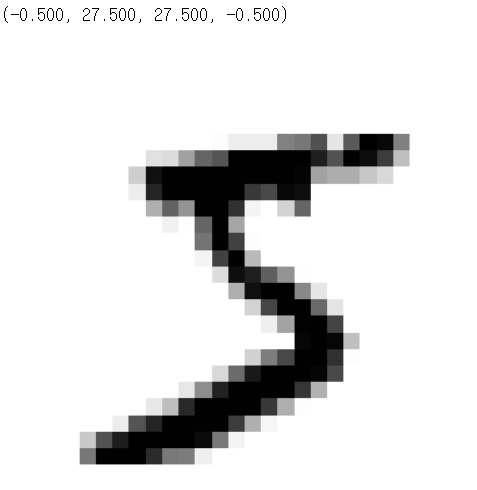
# data load
from sklearn.datasets import fetch_openml
mnist=fetch_openml('mnist_784', version=1, as_frame=False)
print(mnist)
# feature와 target을 분리해보자. X,y=mnist['data'],mnist['target'] # 데이터는 784 픽셀을 가진 흑백 이미지이며, # 실제 크기는 28*28이 된다. # 각 픽셀은 0 ~ 255 까지의 값을 가진다. print(X.shape) print(y.shape)# 이미지 하나를 출력해보자. some_digit=X[0] # 이 이미지는 784 픽셀로 구성 # 2차원 이미지로 변환하자. some_digit_img=some_digit.reshape(28,28) plt.imshow(some_digit_img, cmap=mpl.cm.binary) plt.axis('off')
# 출력한 이미지의 레이블 확인
print(y[0])
#숫자 그림을 위한 추가 함수 #여러 개의 이미지 데이터를 행 단위로 출력하는 함수 #instance는 출력할 이미지, images_per_row는 열의 수 def plot_digits(instances, images_per_row=10, **options): #이미지 크기 설정 size = 28 #열의 개수 설정 images_per_row = min(len(instances), images_per_row) #이미지 전체를 순회하면서 28 * 28로 설정 images = [instance.reshape(size,size) for instance in instances] #행의 개수 구하기 n_rows = (len(instances) - 1) // images_per_row + 1 #이미지 들을 저장할 리스트 row_images = [] n_empty = n_rows * images_per_row - len(instances) #0으로 가득채운 행렬을 만들어서 images 에 저장 images.append(np.zeros((size, size * n_empty))) #행 단위로 순회하면서 이미지를 추가 for row in range(n_rows): rimages = images[row * images_per_row : (row + 1) * images_per_row] row_images.append(np.concatenate(rimages, axis=1)) image = np.concatenate(row_images, axis=0) #이미지 출력 plt.imshow(image, cmap = mpl.cm.binary, **options) plt.axis("off")
- 여러 개의 이미지 출력 함수 확인
plt.figure(figsize=(9,9))
example_images = X[:100]
plot_digits(example_images, images_per_row=5)
save_fig("more_digits_plot")
plt.show()
- 이진 분류를 위한 데이터를 생성하자.
# 훈련 데이터와 테스트 데이터 분리
# mnist는 섞여있다.
X_train, X_test, y_train, y_test= X[:60000], X[60000:], y[:60000], y[60000:]
# 이진 분류는 True와 False로 분류
# 이진 분류의 경우는 Target이 bool
y_train_5=(y_train==5)
y_test_5=(y_test==5)
- sklearn의 SGDClassifier(Stochastic Gradient Descent) - 확률적 경사 하강법 클래스
- 경사 하강법(목표 지점까지 도달하기 위해서 작은 단위로 분할을 한 뒤, 그 분할 단위에서 최선의 방법을 선택)을 이용해서 분류를 처리
- 한 번에 하나씩 훈련 샘플을 선택해서 수행하기에, 데이터의 크기가 수시로 변할 수 있는 온라인 학습에 적합하다.from sklearn.linear_model import SGDClassifier # 훈련에 사용할 모델을 생성 - 하이퍼 파라미터를 설정 # max_iter : 최대 반복 횟수 , max이기에 이 함수는 생각보다 빨리 멈출 수도 있다. # tol 은 정밀도 이다. sgd_clf=SGDClassifier(max_iter=1000,tol=1e-3,random_state=42) # 훈련 sgd_clf.fit(X_train,y_train_5) # 예측 - feature는 2차원 배열 이상이어야 합니다. sgd_clf.predict([some_digit])#5인 데이터를 분류하는 분류기 from sklearn.base import BaseEstimator class Never5Classifier(BaseEstimator): def fit(self, X, y=None): pass def predict(self, X): return np.zeros((len(X), 1), dtype=bool) #분류기 생성 never_5_clf = Never5Classifier() #새로 만든 분류기의 정확도 확인 cross_val_score(never_5_clf, X_train, y_train_5, cv=3, scoring="accuracy")
- 분류의 평가 지표
- 오차 행렬
- 정답이 True와 False로 나누어져 있고, 분류 모델 또한 True와 False의 답을 내놓으면 2*2 행렬로 case를 표현- 이름을 만들 떄는 실제 정답에 관련디 것을 관련된 것을 먼저 부이고, 다음에는 예측한 내용을 붙입니다.
- sklearn에서는 confusion matrix라는
Accuracy(정확도)
- 현재 데이터에서 올바르게 분류한 데이터의 비율
-(TP+TN)/(TP+FN+FP+TN) - 일반적으로 가장 많이 사용하지만, 데이터가 편중된 경우에는 주으이해야 합니다.
- 비올 확률이 99%이고, 안올 확률이 1%인 경우, 무조건 비가 온다고 분류하면 정확도는 99%
Precision(정밀도)
- 모델이 True라고 분류한 것 중에서 실제 True인 것의 비율
TP/(TP+FP)
Recall(재현율)
- 실제 True인 것 중에서 모델이 True라고 예측한 것의 비율
TP/(TP+FN)- 다른 말로는 Sensitivity(민감도) 또는 hit rate라고 합니다.
- 데이터 검색에서 많이 사용하는 지표
F1 Score
- Precision와 Recall의 조화평균
2*((Precision*Recall)/(Precision*recal))- label의 비율이 불균형 구조일 떄 이용합니다.
sklearn에서의 평가 지표 계산
- sklearn.metrics의 서브 패키지의
accuracy_score, precision_score, recall_score, f1_score사용
from sklearn.metrics import accuracy_score, precision_score, recall_score, f1_score
print("accuracy: %.2f" %accuracy_score(y_train_5, y_train_pred))
print("Precision : %.3f" % precision_score(y_train_5, y_train_pred))
print("Recall : %.3f" % recall_score(y_train_5, y_train_pred))
print("F1 : %.3f" % f1_score(y_train_5, y_train_pred))
정밀도와 재현율 트레이드 오프
- 정밀도와 재현율은 서로 상반되는 성질을 가지고 있음
- 정밀도를 높이면, 재현율이 낮아지고, 정밀도를 낮추면 재현율이 높아집니다.
- 이 상황을 정밀도와 재현율 트레이드 오프라고 합니다.
- 분류 모델은 점수나 확류을 가지고 클래스를 결정합니다. - 이진 분류를 // 필기 못함
- 정밀도와 재현율 선택
- 정밀도
ROC Curve(Receiver Operation Characteristic)
-
이진 분류에서 사용하는 도구
-
정밀도 / 재현율 곡선은 정밀도에 대한 재현율 곡선이고, 거짓 양성 비율(FPR)에 대한 진짜 양성 비율(TPR - 재현율)의 곡선
-
FPR
- 1에서 음성으로 정확하게 분류한 음성 샘플의 비율인 음성 비율(True Negative Rate - TNR)를 뺀 값
- TNR을 specificity(특이도) 라고도 한다. -
ROC Curve는 1-특이도 그래프이다.
-
점선이 완전 랜덤 뷴리기
-
점선 으로 부터 멀어지면 멀어질수록 더 좋은 분류기
pr vs roc curve
- 양성 클래스가
✔ 다중 분류
개요
- 2개 이상의 클래스를 분류
- 로지스틱 회귀나 서포트 벡터 머신은 원래 이진 분류만 가능하지만, 이진 분류기를 여러 개 사용하면, 다중 클래스를 분류하는 것이 가능함
- 이진 분류 알고리즘을 이용해서 다중 분류를 가능하게 하는 전략
- 숫자 10개 중 하나를 분류해야 하는 상황이 있을 떄, 10개의 분류기를 만들어서 각 분류기의 점수 중에서 가장 높은 것을 선택하는 방식을 OvR(one_versus-the-rest)또는 OvA(one-versus-all)이라 합니다.
- 모든 조합에 이진 분류기를 훈련시키는 방법은 이를 OVO(one-versus-one)전략이라고 하는데, 클래스가 N개이면 N*(N-1)/2개의 분류기가 빌요함
오차 행렬
- 클래스 개수 만큼의 테이블로 표현 됩니다.
- 다중 분류에서는 오차 행렬을 바로 출력하는 것 보다는 maplotlib의 matshow같은 함수를 이용해서 시각화 하는 것이 효과적이다.
y_train_pred=cross_val_predict(sgd_clf, X_train_scaled, y_train, cv=3)
conf_mx=confusion_matrix(y_train,y_train_pred)
print(conf_mx)
# 오차 행렬을 시각화 plt.matshow(conf_mx,cmap=plt.cm.gray) plt.show()
- 오차 행렬의 결과를 확인해서 오류가 많이 발생하는 특별한 상황이 있다면, 이에 대한 해결책을 제시할 수 있습니다.
- 오류가 많이 발생하는 클래스가 있다면, 그 클래스의 데이터를 조금 더 넣어 모델을 만들거나, 결과가 나온 데이터를 가지고 다시 한 번 학습하는 모델을 만든다거나 전처리 작업을 수행함
# 오차 행렬을 각 행의 합계로 나누고 대각선을 0으로 채워서 오류를 조금 더 눈에 띄게 출력
# 분류 모델에서는 이 행렬을 반드시 출력해보자
# 잘못 분류된 모델을 확인할 수 있기 떄문이다.
row_sums=conf_mx.sum(axis=1, keepdims=True)
norm_conf_mx=conf_mx/row_sums
# 주 대각선 방향을 0으로 채움
np.fill_diagonal(norm_conf_mx,0)
plt.matshow(norm_conf_mx,cmap=plt.cm.gray)
plt.show()
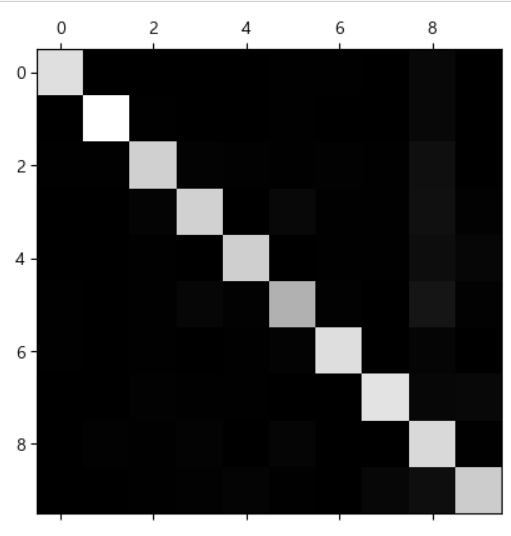
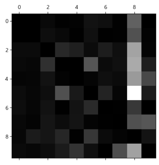
- 이미지의 경우는, 실제 이미지를 출력해서 오류가 발생한 ㅂ누류를 보고, 어떤 전처리를 추가하는 것이 좋을 지 확인해보는 것도 필요합니다.
다중 레이블 분류
- 분류기가 여러 개의 클래스를 출력해야 하는 경우가 발생
- 1개가 아닌 여러 레이블을 분류해서 리턴하는 것을 다중 레이블 분류라고 합니다.
- 얼굴 인식 분류기에서 여러 사람의 얼굴을 식별하는 경우나 객체 탐지 모델의 경우
- KNN을 이용한 다중 레이블 분류
- 평가 지표
- 일반적으로 평균을 내서 사용하면 되는데, 가중치가 있는 경우에는 평가 지표를 구할 때,average='weighted'를 설정해주면 된다.
# 출력해야 할 레이블이 여러 개 인 경우
# 이미지를 가지고 7보다 큰지, 그리고 홀수인지 여부를 같이 리턴하는 경우라면?
from sklearn.neighbors import KNeighborsClassifier
y_train_large=(y_train>=7)
y_train_odd=(y_train%2==1)
# 2개를 가지고 MulitiLabel 생성
y_multilabel=np.c_[y_train_large,y_train_odd]
knn_clf=KNeighborsClassifier()
knn_clf.fit(X_train,y_multilabel)
knn_clf.predict([some_digit])
정리
- 분류 방법
- 이진 분류 : 참과 거짓으로 분류
- 카테고리 분류 : 2개 이상으로 분류
- 다중 레이블 분류 : 결과가 2개 이상인 경우- 평가 지표
- 오차 행렬
- 정확도
- 정밀도, 재현율, F1 Score
- 정밀도와 재현율 트레이드오프(PR)
- ROC 곡선(AUC)- 교차 검증
- 스케일링 작업을 하면 일반적으로 평가지표가 좋아짐
분류 알고리즘
- 대다수의 분류 알고리즘은 회귀에 사용하는 것이 가능
- Target이 범주형이라면, 분류 알고리즘이고, Target이 연속형 숫자라면 회귀 알고리즘이다.
- 앙상블이나 스태킹 알고리즘 1개를 여러 개 쌓거나 여러 개의 알고리즘을 이용하는 방식
판별 분석 (LDA - Linear Discriminant Analysis)
- 2개 이상의 모집단에서 추출된 표본들이 지니고 있는 정보를 이용하여, 이 표본이 어느 모집단에서 추출된 것인지 결정해 줄 수 있는 기준을 찾는 분석법
- 최근에는 평가 지표가 더 높은 알고리즘들이 많이 발견되어서, 직접 사용되는 경우보다는 다른 방법들과 연결되어서 사용하는 경우가 많이 있습니다.
- 용어
- 공분산(covariance) : 하나의 변수가 다른 변수와 함께 변화하는 정도
- 판별 변수(discriminant variable) : 어떤 집단에 속하는지 판별하기 위한 변수로, 독립 변수(feature) 중에서 판별력이 높은 변수를 의미하는데, 상관 관계가 높은 독립 변수들이 존재하는 경우, 이 중 하나만 선택해서 사용하고, 상관 관계가 적은 변수를 선택해서 판별 함수를 생성함
- 판별 함수 : 예측 변수에 적용했을 때, 클래스 구분을 최대화 해주는 함수
- 판별 점수 : 판별 변수의 값을 함수에 대입해서 나온 값 - 선형 판별 분석은 내부 제곱합(그룹 안의 변동을 측정)에 대한 사이 제곱합(그룹 사이의 편차를 측정)의 비율이 최대화 되는 것을 목적
- sklearn.dscriminant.LinearDiscriminantAnalysis 클래스를 이용해서 작업하고 하이퍼 파라미터
# borrowscore 와 pyment_inc_ratio에 따른 columns 선형 판별 분석
loan3000=pd.read_csv('./data/loan3000.csv')
loan3000.head()
loan3000.outcome=loan3000.outcome.astype('category') # 숫자 컬럼들의 상관 계수를 전부 출력 print(loan3000.corr()) # 독립 변수와 종속 변수를 설정 predictors=['borrower_score','payment_inc_ratio'] outcome='outcome' #독립션수 -feature x=loan3000[predictors] # 종속 변수 - target y=loan3000[outcome] print(x) print(y)from sklearn.discriminant_analysis import LinearDiscriminantAnalysis loan_lda = LinearDiscriminantAnalysis() loan_lda.fit(X, y) #최적의 borrower_score 와 payment_inc_ratio 값 구하기 print(pd.DataFrame(loan_lda.scalings_, index=X.columns))# 처음 5개의 데이터 판별 pred=pd.DataFrame(loan_lda.predict_proba(loan3000[predictors])) pred.head() # default와 paid_off의 확률을 확인
KNN(K-Nearest Neighbor - K 최근접 이웃)
- 비선형이며, 분류와 회귀 모두에 사용 가능
- K 개의 유사한 레코드를 찾아서, 가장 많이 채택된 클래스를 할당
- 회귀에 사용되면 그들의 평균을 예측값으로 사용함
- 이웃 : 예측 변수에서 값들이 유사한 레코드(데이터)
- 거리 지표 : 각 데이터들의 거리를 측정하는 방법
- K : 최근접 이웃을 계싼하는데 사용되는 이웃의 개수
- 표준화 : 평균을 뺀 후에 표준편차로 나누는 일
- z 점수 : 표준화를 이용해 나온 값
- 모든 예측 변수들은 수치 값이어ㅑ 함
- 게으른 알고리즘이라고 하는데, 훈련 데이터 세트를 전부 메모리에 저장하고 거리 계산을 수행한다.
from sklearn.neighbors import KNeighborsClassifier
loan200=pd.read_csv('./data/loan200.csv')
# loan200.head()
predictors=['payment_inc_ratio','dti']
outcome='outcome'
newloan=loan200.loc[0:0,predictors]
X=loan200.loc[1:,predictors]
y=loan200.loc[1:,outcome]
print(X)
print(y)
knn=KNeighborsClassifier(n_neighbors=20) # 판별할 이웃의 개수 설정 # 데이터를 가지고 모델을 훈련 knn.fit(X,y) # 예측 print(knn.predict(newloan)) # 확률 확인 print(knn.predict_proba(newloan))
- 표준화
- 독립 변수들의 단위가 차이가 많이 나는 경우, 특정 독립 변수의 영향력이 커지게 됩니다.
- 모든 변수에 평균을 빼고 표준편차로 나누는 과정을 통해서 모두 비슷한 scale이 되도록 하는 것
- 표준화를 수행한 경우와의 차이
loan_data=pd.read_csv('./data/loan_data.csv.gz')
loan_data=loan_data.drop(columns=['Unnamed: 0', 'status'])
loan_data['outcome']=pd.Categorical(loan_data['outcome'],
                                   categories=['paid off', 'default'],
                                   ordered=True)
predictors=['payment_inc_ratio','dti', 'revol_bal', 'revol_util']
outcome='outcome'
# 예측을 위해 떼놓은 데이터 newloan
newloan=loan_data.loc[0:0, predictors]
print(newloan)
X=loan_data.loc[1:, predictors] y=loan_data.loc[1:,outcome] knn=KNeighborsClassifier(n_neighbors=5) knn.fit(X,y) nbrs=knn.kneighbors(newloan) print(X.iloc[nbrs[1][0],:])
- 표준화를 하지 않으면, 이웃을 찾을 때 특정 특성이 영향을 많이 미치게 됩니다.
- 상대적으로 revol_bal이 가까운 데이터가 선택이 되었습니다.
이제 정규화를 해보자.
# 정규화 수행 후 이웃 구하기
from sklearn import preprocessing
scaler=preprocessing.StandardScaler()
scaler.fit(X*1.0) # 정수를 실수로 바꾸면서 정규화
X_std=scaler.transform(X*1.0)
newloan_std=scaler.transform(newloan*1.0)
knn=KNeighborsClassifier(n_neighbors=5)
knn.fit(X_std,y)
nbrs=knn.kneighbors(newloan_std)
print(X.iloc[nbrs[1][0],:])
- 이전에 비해서 revo_bal을 제외한 속성드의 거리들이 가까워졌음
K 선택 (n_neighbors)
- K가 너무 작으면 데이터의 노이즈 성분까지 고려하는 Overfitting 문제가 발생할 수 있고, K가 너무 크면 결정함수가 너무 평탄화 되어서 지역 정보를 예측하는 KNN의 기능을 잃어버리게 됨
- 값을 정하는 규칙은 없고, 데이터에 따라서 적절하게 선택해야 함
- 데이터에 노이즈가 거의 없고 아주 잘 구조화된 데이터의 경우는 k 값이 작을 수록 잘 작동함
- 보통은 1 ~ 20 사이이고, 홀수로 설정
KNN은 구현이 간단하고 직관적(알아보기 쉬움)인데 반해서 성능 면에서는 다른 복잡한 알고리즘에 비해서 떨어지는 편입니다.
- 직접적인 분류나 회귀에 사용하는 것은 어렵지만, 피처 엔지니어링때 많이 사용
- 이 알고리즘을 이용해서 결측치를 치환한다거나, 이를 이용해서 예측 값을 만든 후, 이 값을 다른 모델의 피처로 사용
나이브 베이즈
- 주어진 결과에 대해 예측 변수 값을 확률을 사용해서 추정하는 알고리즘
- 날씨가 맑을 때 경기를 할 확률은?
- 날씨가 맑을 때 경기를 실제로 한 확률만 계산하는 것이 아닌, 날씨가 맑을 확률도 계산에 넣어야 한다는 것이다. - 나이브베이즈에서 확률 계산을 할 때, 정확히 일치하는 레코드로만 제한하지 말고, 전체 데이터를 이용해서 계산을 해야 한다.
- 전체 데이터 14개, 이 중 맑은 날은 4일
- 전체 데이터에서 경기를 한 날은 9일, 맑은날 중 경기를 한 날은 4일
- 단순히 보면 그냥 100%이다.
- 나이브 베이즈 사전 확률
- 맑은 날 : 4/14 : 0.29
- 경기 : 9/14 : 0.64- 나이브 베이즈 사후 확률
- 맑은 날의 개수를 경기를 한 날로 나누기
- 4/9 : 0.44- 베이즈 공식에 대입하기
- 0.44*0.64/0.29 = 0.98
Logistic Regression
- 이름은 회귀지만, 분류에만 사용 가능
- Odds Ratio(특정 이벤트가 발생할 확률) 이용
-Odds Ratio=성공율/실패율=성공율/(1-성공율) - Logit 함수
- Odds Ratio에 자연 로그를 취한 값
- 값의 범위를 0 ~ 1로 입력받아서 자연 로그를 취한 함수
- 샘플이 특정 클래스에 속할 확률을 예측하는 것이 목적이므로, 실제 사용은 logit 함수를거꾸로 뒤집는데 이 함수를 로지스틱 시그모이드함수라고 한다. - 시그모이드 함수는 단순 선형이 아니라서, 아무래도 단순 헌형 회귀보다는 잔차가 적을 확률이 높다.
- Iris 데이터 : 분류에 사용
- Sepal Length
- Sepal Width
- Petal Length
- Petal Width
- Species : 꽃의 종류 (setosa/versicolor/virginica) - LogisticRegression의 Hyper Parameter
- penalty: l1,l2
- dual : Daul Formulation인지 Primal Formulation인지 설정하는데 bool
- tol : 중지 기준에 대한 오차 허용 값
- C : 규칙 강도의 역수 값(penalty와 같이 다님)
- fit_intercipt : 의사 결정 기능에 상수를 추가할 지 여부로 bool
- class_weight : 클래스들에 대한 가중치
- random_state
- solver : 최적화에 사용할 알고리즘(newton-cg, lbfgs, liblinear, sag, saga)
- max_iter : solver가 수렴하게 만드는 최대 반복 횟수 값
- multi_class : ovr인지 multinomial
- warm_start : 이전 호출에 사용한 solution을 재사용할 지 여부
- n_jobs : 병렬 처리 시 사용할 CPU 코어의 수(-1 : 모든 비트 값이 1 ) 이면 최대치 - 붓꽃의 이진 분류를 해보자.
- virginica인지 여부를 판단해보자.
# 데이터 가져오기
from sklearn import datasets
iris=datasets.load_iris()
# list(iris.keys())
# 피쳐 생성
X=iris['data'][:,3:]
y=(iris['target']==2).astype(np.uint8)
# print(X)
# print(y)
from sklearn.linear_model import LogisticRegression #분류 모델 생성 log_reg=LogisticRegression(solver='lbfgs',random_state=42) # 모델 훈련 log_reg.fit(X,y) #샘플 데이터를 1000개 생성해서 예측하기 X_new=np.linspace(0,3,1000).reshape(-1,1) # 각 샘플의 확률 계산 y_proba=log_reg.predict_proba(X_new) # 경계점수 decision_boundary=X_new[y_proba[:,1]>=0.5][0] print(decision_boundary) # 예측 print(log_reg.predict([[1.7],[1.5]]))
- 로지스틱 회귀 모델도 선형 모델이기 때문에 규제가 가능합니다.
- 기본적으로 sklearn은 l2 규제를 사용하는데, l1규제로 변경 가능
- 규제 강도를 모델을 만들 떄, C를 이용해서 규제의 강도를 설정할 수 있는데, alpha가 아니고 C인 이유는 역수를 취하기 때문이다.
- 모델의 규제를 높이면, 모델의정확도는 높아지지만, Overfitting(훈련 데이터에는 잘 맞지만, 새로운 데이터에는 잘 맞지 않을 가능성이 높아지는 것) 될 가능성이 존재하고, 규제를 낮추면 Overfitting 가능성은 낮아지지만, Underfitting(훈련 데이터에 잘 맞지 않는 상황) 가능성이 높아집니다.

밀가루 귀여워요