수업 41일차

✔ Machine Learning

일반화에 따른 분류

사례 기반 학습

• 사례 기반 학습은 단순히 기억하는 것
• 스팸 메일 필터를 만드는 경우
  - 사용자가 스팸이라고 지정한 메일과 동일한 모든 메일을 스팸으로 분류
  - 다른 메일을 스팸이라고 판정을 하려면 일단 메일과 메일 사이의 유사도(거리)를 측정
  - 일반적인 거리 측정 방법은 공통된 단어의 개수를 세는 것
  - 스팸 메일과 공통된 단어가 많으면 스팸으로 간주하는 방식
  - 사례를 기억해서 그 사례와 유사성을 살펴서 새로운 데이터에 일반화 시키는 방식
• KNN이 대표적인 모델

모델 기반 학습

• 훈련 데이터를 가지고 모델을 만들어서 이 모델을 이용해서 새로운 데이터를 예측
• 돈이 사람을 행복하게 만드는지 알아보고자 하는 경우
  - 돈을 독립 변수로 해서 행복 지수를 찾아내는 것
  - 행복 지수는 실수이므로 회귀 분석을 수행
  - 회귀 분석을 수행하면 하나의 식이 완성
  - 선형회귀라면 행복지수=돈*가중치+상수
  - 새로운 데이터가 제공되면 수식에 대입해서 행복 지수를 산출
  

모델 평가 방법

잔차(에러)의 제곱

• 회귀 분석에 사용
• 회귀식에 의해서 계싼된 값과 실제 값의 차이 (잔차)
• 모든 데이터의 잔차를 전부 찾아서 제곱한 하고 더한 값
• 대부분의 회귀 분석 모델은 잔차의 제곱이 작은 쪽으로 학습

Accuracy(정확도)

• 정확하게 분류한 개수 / 전체 데이터 개수
• 분류 분석에 사용

Likehood(우도, 가능도)

• 확률 분포의 모수가 어떤 확률 변수의 표본 값과 일관되는 정도를 나타내는 값
• 확률 추정 모델에 사용

Precision(정밀도)

• 내가 원하는 결과의 확률로 정보 검색에서 많이 이용함
• 100개의 검색 결과가 제공되었을 때, 내가 원하는 결과가 80개라면 정밀도는 0.8

Recall(재현율)

• 전체 데이터 중 얼마나 제대로 검색했는지를 확인
• 전체 데이터가 100개 인데, 구글이 40개를 검색했다면 재현율은 0.4

Entropy

• 정답 레이블의 확률과 예측한 확률과의 거리
• 분류에서 사용함

데이터

복잡한 문제에서는 알고리즘 보다는 데이터의 양이 훨씬 더 중요함

대표성이 없는 훈련 데이터

• 샘플링 데이터가 너무 적으면 샘플링 잡음(Sampling Noise)이 발생함
• 샘플이 많은 경우에도 샘플링 방법이 잘못되었다면, 샘플링 편향(Sampling Bias)이 발생함

낮은 품질의 데이터

• 에러, 이상치, 잡음의 비율이 높은 데이터
• 이런 경우에는 정제를 수행하고 학습해야 한다.

관련없는 특성

• Garbage in Garbage Out
  - 입력이 잘모된다면 잘못된 결과가 도출될 것이다.
• 특성 공학(Feature Engineering) : 훈련에 사용할 좋은 특성을 찾는 것
  - 특성 선택
  - 특성 추출 : 특성을 결합해서 새로운 특성을 생성 - 차원 축소
  - 새로운 데이터를 수집해서 새로운 특성 생성
  

훈련 데이터 과대 적합(Overfitting)

• 훈련 데이터에는 잘 맞지만, 일반성이 떨어지는 경우
• 훈련 데이터에 잡음이 많은 경우에 주로 발생
• 행복 지수를 계산하고자 하는 경우에, 나라 이름을 포함해서 행복 지수를 산출

Newziland - 7.3
Norway - 7.4
Sweden - 7.2
Swiss - 7.5
-> Rwanda를 예측해보자.

• 해결 기법
  - 파라미터 수를 줄인 모델을 선택 : 고차원 다항 모델보다는 선형 모델을 선택
  - 훈련 데이터의 특성 수를 줄이거나 모델에 제약(규제)를 가함
  - 훈련 데이터를 많이 수집함
  - 정제를 통해서 잡음을 줄임

과소 적합(Underfitting)

• 모델이 너무 단순해서 데이터의 내재된 구조를 학습하지 못하는 경우
• 해결 기법
  - 파라미터가 많은 더 강력한 모델을 선택
  - 학습 알고리즘에 더 좋은 특성을 제공
  - 모델의 제약을 줄임
  

Test & Validation

• 모델을 평가하는 가장 좋은 방법은, 실제 서비스에 모델을 넣고 잘 작동하는지 확인하는 것
  - 현실적으로 불가능
• 샘플을 분리해서 일부분은 모델을 만드는데 사용하고 나머지를 가지고 테스트를 수행
  - 3가지 또는 2가지로 분류
• 훈련 데이터
  - 모델을 만드는 데 사용하는 데이터
• 테스트 데이터
  - 모델을 테스트하기 위한 데이터로, 이 데이터로 모델을 수정
• 검증 데이터
  - 만들어진 모델을 확인하기 위한 데이터
• 8:2, 7:3, 7:2:1 을 많이 사용하는데, 이 비율은 개발자가 선택
• 데이터가 아주 많은 경우에는, 훈련 데이터의 비중을 낮추기도 합니다.

하피어 파라미터 튜닝

• Parameter
  - 모델 내부에서 결정되는 변수

• 선형 회귀를 하게 된다면, 기울기와 절편이 나오게 됩니다.

• 기울기와 절편은 입력된 데이터에 의해서 결정됩니다.

• 이런 값들을 매개변수라고 합니다.

• Hyper Parameter : 개발자가 결정하는 변수
  - 모델을 만들 때, 입력하는 데이터
  - 모델의 성능이 좋지 못하다면, 하피어 파라미터를 수정해서 모델의 성능을 좋은 쪽으로 수정
  

• 홀드 아웃 검증
  - 샘플링 된 데이터에서 일부분을 선택해서 여러 모델을 평가하고, 가장 좋은 하나를 선택하는 방식
  - 검증을 위한 데이터의 크기가 너무 작다면, 모델이 정확하게 평가되지를 않아서, 최적이 아닌 모델을 선택할 수 있으며, 검증을 위한 데이터가 너무 크다면 훈련 데이터의 양이 작아지게 되는 효과를 발생함
  - 작은 검증 세트를 여러 개 만들어서 반복적인 교차 검증을 수행하는 것을 권장함
  

✔ Scikit Learn을 이용한 머신 러닝

Scikit Learn

• anaconda에는 이미 설치가 되어있으며, python에는 없기 때문에 python을 사용하는 경우에는 설치
• python 기반의 Machine Learning을 위한 가장 쉽고 효율적인 개발 라이브러리
• 최근에는 Keras, Tensorflow, Pytorch등의 딥러닝 라이브러리도 많이 사용함

특징

• 가장 python 스러운 api를 제공함
• 오랜 기간 실전에서 사용이 된 라이브러리
• ML을 위한 다양한 알고리즘과 개발을 위한 편리한 프레임워크와 API를 제공함

데이터 표현 방식

• 테이블 구조
  - numpy의 배열이나 pandas의 DataFrame을 사용
  

#머신러닝에 사용할 데이터 가져오기
import seaborn as sns
iris = sns.load_dataset('iris')
iris.info()
# feature matrix 와 target을 분리
X_iris = iris.drop('species', axis=1)
y_iris = iris['species']
print(X_iris.shape)
print(y_iris.shape)

• 하나의 행을 Sample이라고 부르고, 전체를 표본(Sample)이라고 하며, 행의 개수를 n_samples라고 합니다.
• 하나의 열은 feature나 target이라고 부르며, 열의 개수를 n_features라고 합니다.
• 전체 데이터를 feature matrix(특징 행렬)이라고도 부르며, 대부분의 경우에는 numpy의 ndarray나 pandas의 DataFrame이지만 특별한 경우에는 sparse matrix로 만들기도 합니다.
  target이 없는 featrue matrix는 관례상 X로 사용
• target은 관례상 y로 사용하고 numpy의 일차원 배열이나 pandas의 Series로 제공

API 이용 과정

• 적절한 estimator(추정기 - 모델) 클래스를 import해서 모델의 클래스를 선택
• 클래스를 원하는 값으로 인스턴스화해서 hyperparameter를 선택
• 데이터(feature matrix와 target)를 배치
• fit 메서드를 이용해서 훈련
• 모델을 새로운 데이터에 적용
  - 지도 학습의 경우는 predict()를 이용함
  - 비지도 학습에서는 transform이나 predict 함수를 이용
• 데이터를 생성해서 선형 회귀를 수행

# 선형 회귀 수행
#1.데이터 수집
rng = np.random.RandomState(42)
X = 10 * rng.rand(50)
y = 2 * X - 1 + rng.randn(50)
plt.scatter(X, y)
#2.모델을 선택하고 인스턴스를 생성
from sklearn.linear_model import LinearRegression
model = LinearRegression(fit_intercept = True)
print(model)
#3.모델 훈련
#특징 벡터는 2차원 배열이어야 합니다.
#1차원 배열을 2차원 배열로 변경하고자 하면 reshape를 이용해도 되고
#열을 하나 추가해서 2차원으로 만들어도 됩니다.
#여기서는 2차원으로 변경
print(X.shape)
print(X[:, np.newaxis].shape)
model.fit(X[:, np.newaxis], y)
print(model.coef_) #기울기 - slope
print(model.intercept_) #절편 - intercept
#4.예측
#예측에 사용할 데이터 생성
X_fit = np.linspace(-1, 11)
Xfit = X_fit[:, np.newaxis]
yfit = model.predict(Xfit)
#print(yfit)
plt.scatter(X, y)
plt.plot(Xfit, yfit)

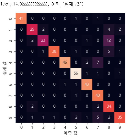
숫자 이미지를 분류해보자.

#1.데이터 수집
from sklearn.datasets import load_digits
digits = load_digits()
print(digits.images.shape)

#2.데이터 확인 - 이미지 출력
#print(digits.images[0])
fig, axes = plt.subplots(10, 10, figsize=(8, 8),
                         subplot_kw={'xticks':[], 'yticks':[]},
                        gridspec_kw=dict(hspace=0.1, wspace=0.1))
for i, ax in enumerate(axes.flat):
    ax.imshow(digits.images[i], cmap='binary', interpolation='nearest')
    ax.text(0.05, 0.05, str(digits.target[i]), transform=ax.transAxes, color='green')

#3.특징 배열 과 타겟을 생성
X = digits.data
print(X.shape)
y = digits.target
print(y.shape)
#훈련 데이터 와 테스트 데이터 분리
from sklearn.model_selection import train_test_split
#별다른 옵션이 없으면 75:25 로 분할
Xtrain, Xtest, ytrain, ytest = train_test_split(X, y, random_state=42)
print(Xtrain.shape)
print(Xtest.shape)
help(train_test_split)

#4.분류 모델을 선택해서 훈련
from sklearn.naive_bayes import GaussianNB
model = GaussianNB()
model.fit(Xtrain, ytrain)
#예측
y_model = model.predict(Xtest)

#5.정확도 확인
from sklearn.metrics import accuracy_score
#실제 값 과 예측한 값을 대입해서 정확도 확인
accuracy_score(ytest, y_model)
#6. 오차 행렬
from sklearn.metrics import confusion_matrix
mat = confusion_matrix(ytest, y_model)
#print(mat)
sns.heatmap(mat, square=True, annot=True, cbar=False)
plt.xlabel('예측 값')
plt.ylabel('실제 값')

#7. 실제 이미지에서 잘못 분류된 데이터 확인
fig, axes = plt.subplots(10, 10, figsize=(8, 8),
                         subplot_kw={'xticks':[], 'yticks':[]},
                        gridspec_kw=dict(hspace=0.1, wspace=0.1))
test_images = Xtest.reshape(-1, 8, 8)
#제대로 분류된 경우는 녹색 그렇지 않은 경우는 빨강색으로 화면에 텍스트 출력
for i, ax in enumerate(axes.flat):
    ax.imshow(test_images[i], cmap='binary', interpolation='nearest')
    ax.text(0.05, 0.05, str(digits.target[i]), transform=ax.transAxes, 
            color='green' if (ytest[i] == y_model[i]) else 'red')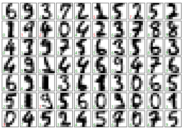

PCA(주성분 분석) - 차원 축소

• 여러 개의 차원을 합쳐서 하나의 새로운 차원을 만드는 것
• 각 특성을 가지고 모델을 만들었을 때, 모델의 성능이 좋지 못하르 때, 여러 개의 차원을 줄여서 사용하면 모델의 성능이 좋아질 수 있습니다.
• 특성이 너무 많으면 overfitting 될 가능성이 높습니다.
• 이 경우는 오차의 개념이 없습니다.
• 비지도 학습이므로 정답이 없습니다.
  - 모델을 만들기 위해서 하는 것이 아닌, 모델의 성능을 높이기 위해서 수행하는 것입니다.

from sklearn.decomposition import PCA
model = PCA(n_components=2) # 2개의 주성분
model.fit(X_iris) #이 경우는 훈련 데이터 와 테스트 데이터를 분할하지 않음
X_2D = model.transform(X_iris)
#주성분 결과를 원본 데이터에 반영
iris['PCA1'] = X_2D[:, 0]
iris['PCA2'] = X_2D[:, 1]
sns.lmplot(x="PCA1", y="PCA2", hue='species', data=iris, fit_reg=False)

Clustering(군집) - 비지도 학습

• 비지도 학습이지만 predict를 수행함

from sklearn.mixture import GaussianMixture
model = GaussianMixture(n_components=3, covariance_type='full')
model.fit(X_iris)
y_gmm = model.predict(X_iris)
iris['cluster'] = y_gmm
print(iris)

• 비지도 학습은 훈련 데이터 외 테스트 데이터를 분할하지 않음
  - 없는 레이블을 만드는 것이므로, 비교할 레이블이 없어서 옳고 그름을 판단할 근거가 없음

✔ 머신러닝의 수행 절차

1. 문제 정의
2. 작업 환경 설정
3. 데이터 수집
4. 데이터 탐색
5. 전처리
6. 모델을 선택해서 훈련
7. 모델을 상세하게 조정
8. 솔루션을 제시
9. 시스템을 론칭하고 모니터링하면서 유지 보수

✔ 머신러닝 수행

문제 정의

• 캘리포니아 인구 조사 데이터(housing.csv)를 이용해서 캘리포니아 주택 가격 모델을 생성
• 주택 가격 에측
• 주택 가격을 가지고 있으므로, 지도학습이다.
• 주택 가격은 범주형 데이터가 아니기에, 회귀분석이다.
• 변수가 여러개라서 다변량 회귀 분석이다.
• 새로운 데이터가 입력되는 구조가 아니라서 배치학습이다.
  - 새로운 데이터가 주기적으로 입력되는 구조라면, 온라인 학습으로 처리
  

데이터 수집

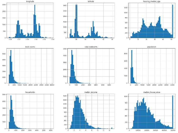
import pandas as pd
#1.데이터 가져오기
housing = pd.read_csv('./data/housing.csv')
print(housing.head())

데이터 탐색

housing.info()
#총 데이터 개수는 20640개
#속성은 10개
#ocean_proximity 을 제외하고는 전부 실수
#total_bedrooms 은 결측치 존재
#범주형 가능성이 있는 데이터를 확인
print(housing['ocean_proximity'].value_counts())
#값이 5가지만 존재하므로 범주형일 가능성이 높음
#기술 통계량 확인
housing.describe()
#데이터의 분포 확인
housing.hist(bins=50, figsize=(20, 15))
#이미지 저장
plt.savefig('histogram', format='png', dpi=300)
plt.show()

• 데이터의 분포를 확인해서, 꼬리가 길고 한쪽으로 많이 쏠려있는 데이터의 경우는 패턴을 찾기 어렵기 때문에, 좀 더 종의 분포가 되도록 조정할 필요가 있음
• 각 속성의 단위가 다르다면, 좋은 모델이 만들어지기 어렵기 때문에 스케일링을 고려해야 한다.

테스트 데이터 만들기

• 전체 데이터를 가지고 모델을 만들면, 과대 적합되기 쉬운 상황이 발생함
• 일반화 오차를 추정해보면, 매우 낙관적인 추정이 되어서 시스템을 실제 론칭을 하게 된다면 기대한 성능이 나오지 않는 것이 일반적 - Data Snooping
• 테스트 데이터를 20% 정도 분리시켜서 모델을 만들고 난 후 이 데이터를 이용해서 검증하는 것을 권장
• 무작정 랜덤하게 샘플링을 하면 안되는데, 프로그램을 실행할 때 마다 다른 테스트 세트가 생성되고, 이를 반복하면 결국 알고리즘이 전체 데이터를 가지고 만들어지기 때문
• 별도의 테스트 데이터를 다른 곳에 저장하고, 테스트를 수행할 때, 불러들이는 방식으로 만들거나 난수를 생성하는 seed값을 고정시키는 형태로 만들면 위와 같은 상황을 방지할 수 있습니다.

#시드를 고정
np.random.seed(42)
#데이터 와 테스트 데이터의 비율을 매개변수로 받아서 테스트 데이터를 리턴해주는 함수
def split_train_test(data, test_ratio):
    #랜덤한 숫자 인덱스를 생성
    shuffled_indices = np.random.permutation(len(data))
    #테스트 데이터의 크기 결정
    test_set_size = int(len(data) * test_ratio)
    test_indices = shuffled_indices[:test_set_size]
    train_indices = shuffled_indices[test_set_size:]
    return data.iloc[train_indices], data.iloc[test_indices]
train_set, test_set = split_train_test(housing, 0.2)
print(len(train_set), len(test_set))

• 이전 방식으로 데이터를 가져오는 경우, 데이터의 개수가 변경되면, 다른 데이터가 테스트 데이터가 됩니다.
• 온라인 학습 또는 데이터가 주기적으로 변경되는 경우, 이 방식은 문제가 발생할 소지가 있습니다.
  - 고정된 데이터