제로베이스 데이터취업스쿨 DAY64-77 통신사이탈고객예측 전처리

import pandas as pd 
import numpy as np 
import matplotlib.pyplot as plt
import seaborn as sns 
import koreanize_matplotlib # 한글설정 라이브러리 
import plotly.express as px
import collections

from sklearn.preprocessing import LabelEncoder
from sklearn.preprocessing import RobustScaler
from sklearn.ensemble import IsolationForest
from sklearn.decomposition import PCA
from imblearn.over_sampling import SMOTE

%matplotlib inline

train = pd.read_csv('cell2celltrain.csv')
test = pd.read_csv('cell2cellholdout.csv')

기본 전처리

결측치 처리

data1 = train.copy()
data1.isnull().sum().sort_values(ascending=False)

data1.dropna(inplace=True)
data1.reset_index(drop=True, inplace=True)

라벨인코딩

• 범주형 컬럼 중 'CustomerID', 'HandsetPrice' 제거 후 라벨인코딩

data1.drop(columns=['CustomerID', 'HandsetPrice'], inplace=True, axis=1) 
le = LabelEncoder()
object_cols = data1.select_dtypes(include=['object']).columns
data1[object_cols] = data1[object_cols].apply(le.fit_transform)

data1.to_csv('data1.csv', index=False)

case3 이후 데이터 전처리

data2 = train.copy()

결측치 제거

data2.dropna(inplace=True)
data2.reset_index(drop=True, inplace=True)
data2.isnull().sum().sort_values(ascending=False)

Homeownership, Handsetprice, MaritalStatus, ServiceArea 컬럼 제거

• Unknown 값이 50% 이상인 컬럼과 ServiceArea 제거

drop_cols = ['MaritalStatus', 'HandsetPrice', 'Homeownership', 'ServiceArea' , 'CustomerID']
data2.drop(drop_cols, inplace=True, axis=1)

AgeHH1, AgeHH2의 0값은 소득 그룹과, 신용등급이 동일한 그룹의 중간값으로 대치

cond1 = (data2[['AgeHH1']]!=0).values
cond2 = (data2[['AgeHH2']]!=0).values
data_not_zero =  data2[cond1&cond2]
grouped_median = data_not_zero.groupby(['IncomeGroup', 'CreditRating'])[['AgeHH1', 'AgeHH2']].agg('median')

for index, row in data2.iterrows():
    if row['AgeHH1'] == 0:
        median_value = grouped_median.loc[(row['IncomeGroup'], row['CreditRating']), 'AgeHH1']
        data2.at[index, 'AgeHH1'] = median_value
    
    if row['AgeHH2'] == 0:
        median_value = grouped_median.loc[(row['IncomeGroup'], row['CreditRating']), 'AgeHH2']
        data2.at[index, 'AgeHH2'] = median_value
        
def draw_px_histogram(df, x):
    fig = px.histogram(df, x=x)
    fig.update_layout(
    width=1500,  
    height=500, 
    )
    fig.show()

라벨인코딩

le = LabelEncoder()
object_cols = data2.select_dtypes(include=['object']).columns
data2[object_cols] = data2[object_cols].apply(le.fit_transform)

이상치 제거

# n_estimators : 노드 수 (50 - 100사이의 숫자면 적당하다.)
# max_samples : 샘플링 수
# contamination : 이상치 비율
# max_features : 사용하고자 하는 독립변수 수 (1이면 전부 사용)
# random_state : seed를 일정하게 유지시켜줌(if None, the random number generator is the RandomState instance used by np.random)
# n_jobs : CPU 병렬처리 유뮤(1이면 안하는 것으로 디버깅에 유리. -1을 넣으면 multilple CPU를 사용하게 되어 메모리 사용량이 급격히 늘어날 수 있다.)

clf_ss = IsolationForest(n_estimators=100,
                      max_samples="auto", 
                      contamination=0.01,
                      max_features=1,
                      bootstrap=False,
                      n_jobs=1,
                      random_state=None,
                      verbose=0)

# fit 함수를 이용하여, 데이터셋을 학습시킨다.
clf_ss.fit(data2)

# predict 함수를 이용하여, outlier를 판별해 준다. 0과 1로 이루어진 Series형태의 데이터가 나온다.
y_pred_outliers = clf_ss.predict(data2)

# 이상치의 개수를 Count하는 과정
collections.Counter(y_pred_outliers)

# 원래의 DataFrame에 붙히기. out행의 값이 -1인 것을 제거하면 이상치가 제거된 DataFrame을 얻을 수 있다.
data2['out']=y_pred_outliers
outliers=data2.loc[data2['out']== -1]
outlier_index=list(outliers.index)

pca = PCA(2)
pca.fit(data2)
res=pd.DataFrame(pca.transform(data2))
Z = np.array(res)
plt.title("IsolationForest")
b1 = plt.scatter(res[0], res[1], c='green',
                 s=20,label="normal points")
b1 =plt.scatter(res.iloc[outlier_index,0],res.iloc[outlier_index,1], c='green',s=20,  edgecolor="red",label="predicted outliers")
plt.legend(loc="upper right")
plt.show()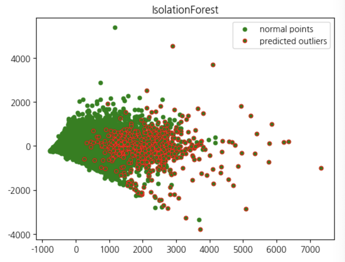

train_rm_out = data2[data2['out'] != -1]
train_rm_out['Churn'] = data2["Churn"]

RobustScaler

def scale_data_with_robust_scaler(data):
    rs = RobustScaler()
    scaled_data = pd.DataFrame(rs.fit_transform(data), columns=data.columns)
    return scaled_data

오버샘플링

# Separate features (X) and target variable (y)
X = train_rs.drop('Churn', axis=1)
y = train_rs['Churn']

# Apply SMOTE to balance the target variable
smote = SMOTE(random_state=70)
X_resampled, y_resampled = smote.fit_resample(X, y)

# Create a new DataFrame with the balanced data
train_ss_ov = pd.concat([X_resampled, y_resampled], axis=1)