해당 글은 제로베이스데이터스쿨 학습자료를 참고하여 작성되었습니다
타이타닉 생존자분석
개요
- 영화의 마지막 장면에 판자에 위즐렛을 남겨놓고 죽은 디카프리오에 대해서 말이 많았다
- 판자 위에 같이 있었다면 죽지 않을 것이라는 말이 있었다
- 데이터분석을 통해서 디카프리오가 생존할 수 있었는지 예측해보자
목표
- 디카프리오 생존율 예측하기
절차
- 데이터 이해
- 생존율 분석
- 타이타닉의 진실
- DecisionTree 활용
- 주인공 생존율 예측
타이타닉 데이터 가져오기
import pandas as pd

titanic_url='https://raw.githubusercontent.com/PinkWink/ML_tutorial/master/dataset/titanic.xls'

titanic = pd.read_excel(titanic_url)
titanic.head()
1) 데이터 이해
칼럼 확인
- pclass : 객실등급
- survived : 생존유무
- sex : 성별
- age : 나이
- sibsp : 형제 혹은 부부의 수
- parch : 부모 혹은 자녀의 수
- fare : 지불한 요금
- boat : 탈출을 했다면 탑승한 보트의 번호
2) 생존율 분석
전체 생존율
import matplotlib.pyplot as plt
import seaborn as sns
from matplotlib.pyplot import rc, rcParams

%matplotlib inline
rc('font', family='Malgun Gothic')
rcParams['axes.unicode_minus'] = False
titanic['survived'].value_counts()
-----------------------------------------------
0    809
1    500
Name: survived, dtype: int64f, ax = plt.subplots(1, 2, figsize=(16, 8))
# 좌측 Pie plot
titanic['survived'].value_counts().plot.pie(ax = ax[0], autopct='%1.1f%%', shadow=True, explode=[0, 0.05]);
ax[0].set_title('Pie plot - survived')
ax[0].set_ylabel('')
# 우측 Count plot
sns.countplot(data=titanic, x='survived', ax = ax[1])
ax[1].set_title('Count plot - survived')
# bar 위에 수치 표기
for p in ax[1].patches:
height = p.get_height()
ax[1].text(p.get_x() + p.get_width() / 2., height + 3, height, ha = 'center', size = 9)
plt.show()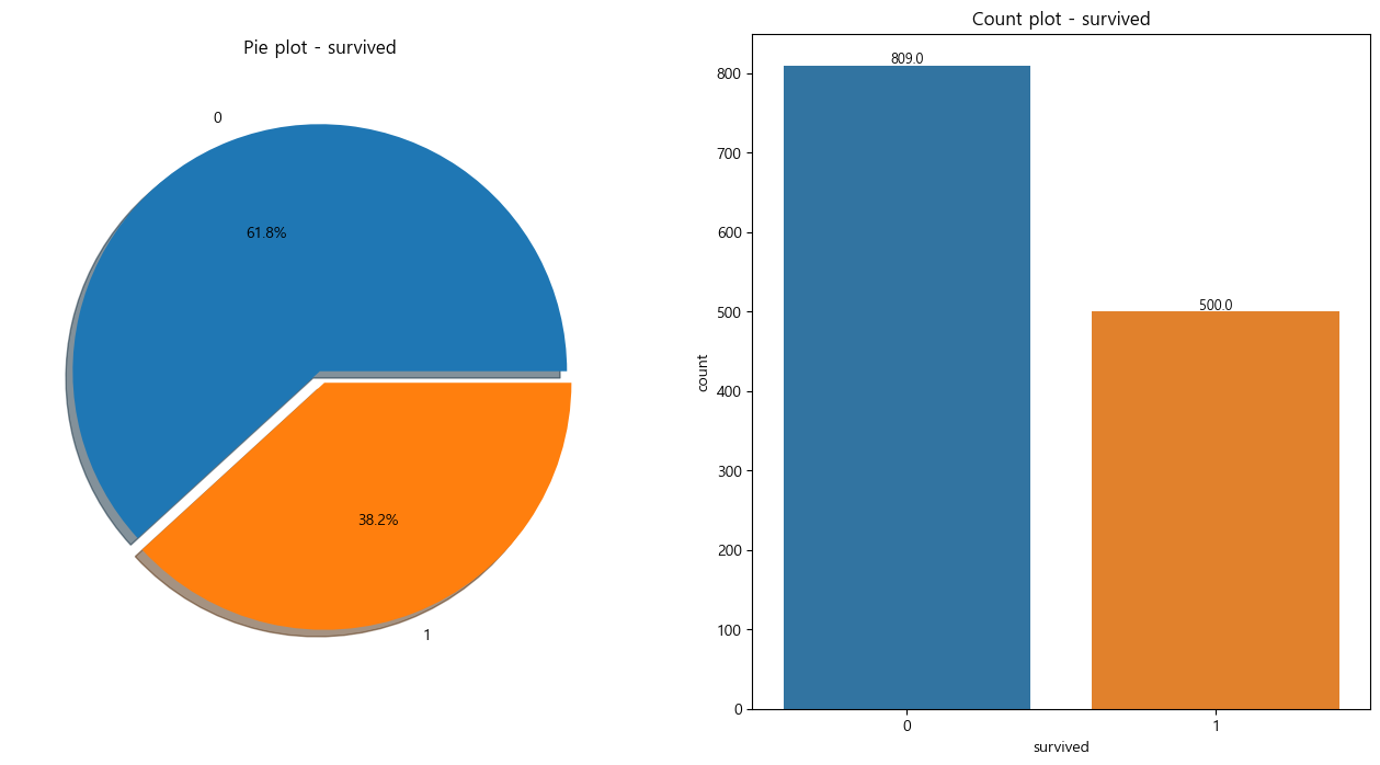
생존율 확인결과
- 생존율 : 38.2%
- 사망율 : 61.8%
- 생존수 : 500명
- 사망수 : 809명
성별 생존율
# 성별에 따른 생존 데이터
fig, ax = plt.subplots(1,2, figsize=(18,8))

# 좌측 Pie plot
sns.countplot(data=titanic, x='sex', ax=ax[0])
ax[0].set_title('Count of Passengers of Sex')
ax[0].set_ylabel('')
for p in ax[0].patches:
    height = p.get_height()
    ax[0].text(p.get_x() + p.get_width() / 2., height + 3, height, ha = 'center', size = 9)

# 우측 Count plot
sns.countplot(data=titanic, x='sex', hue='survived', ax=ax[1])
ax[1].set_title('Sex : Survived')
for p in ax[1].patches:
    height = p.get_height()
    ax[1].text(p.get_x() + p.get_width() / 2., height + 3, height, ha = 'center', size = 9)

plt.show()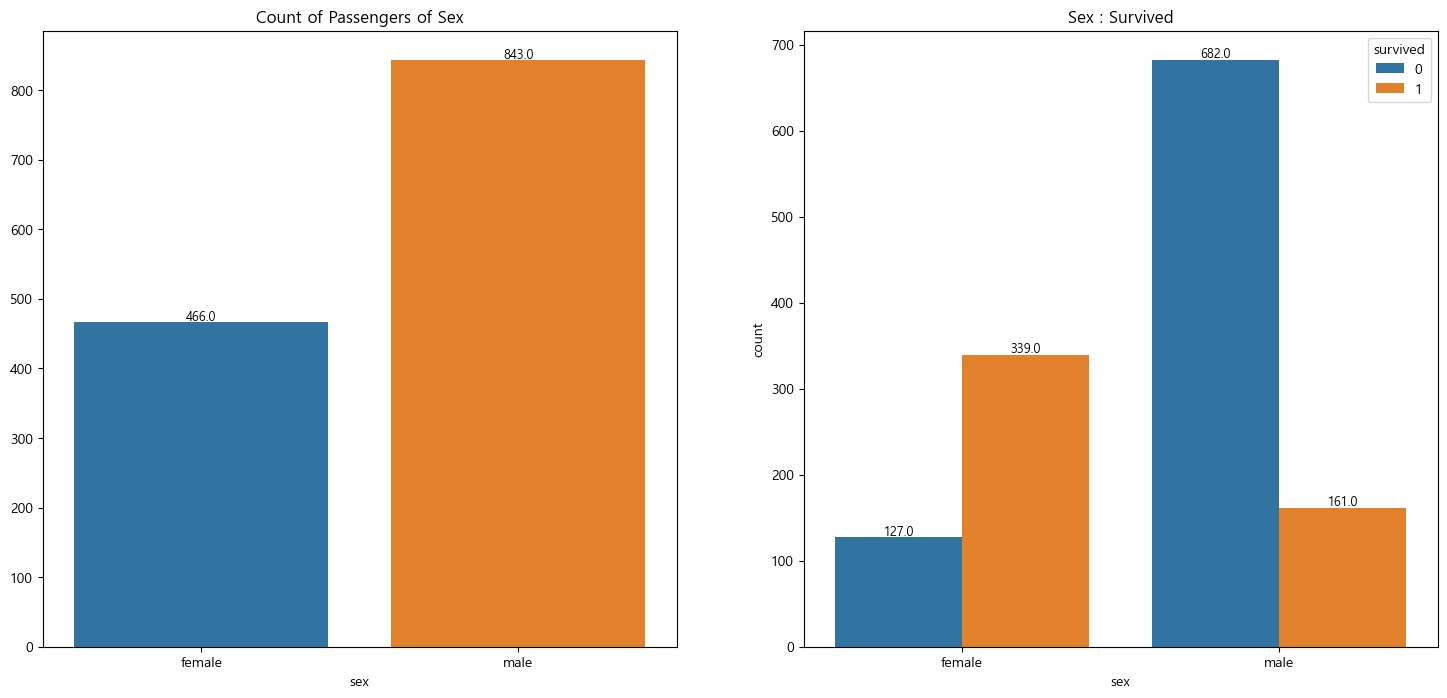
성별 생존율 확인결과
- 탑승객 : 남성(843명) + 여성(466명) = 1309명
- 사망자
- 여성 : 466명 중 127명 사망, 27%
- 남성 : 843명 중 682명 사망, 81%
- 남성의 사망 비율이 상당히 높다
- 지금까지의 정보만 보았을 때, 남성이 더 많으므로 생존율 또한 남성이 더 많아야 한다
- 하지만 그렇지 않은데 그 이유를 파악하기 위해 좀 더 알아보자
경제력에 따른 생존데이터 시각화
df = pd.crosstab(titanic['pclass'], titanic['survived'], margins=True)
df['Death Pct'] = round(df[0]/df['All'], 2)
df
------------------------------------------------------------------------
survived    0    1   All  Death Pct
pclass
1         123  200   323       0.38
2         158  119   277       0.57
3         528  181   709       0.74
All       809  500  1309       0.62
경제력 생존데이터 확인결과
- 1등실 사망율 : 323명 중 123명 사망, 38%
- 2등실 사망율 : 277명 중 158명 사망, 57%
- 3등실 사망율 : 709명 중 528명 사망, 74%
선실등급과 성별에 따른 나이분포 데이터
# 탑승객의 정보
grid = sns.FacetGrid(titanic, row='pclass', col='sex', height=4, aspect=2)
grid.map(plt.hist, 'age', alpha=0.8, bins=20)
grid.add_legend()
plt.show()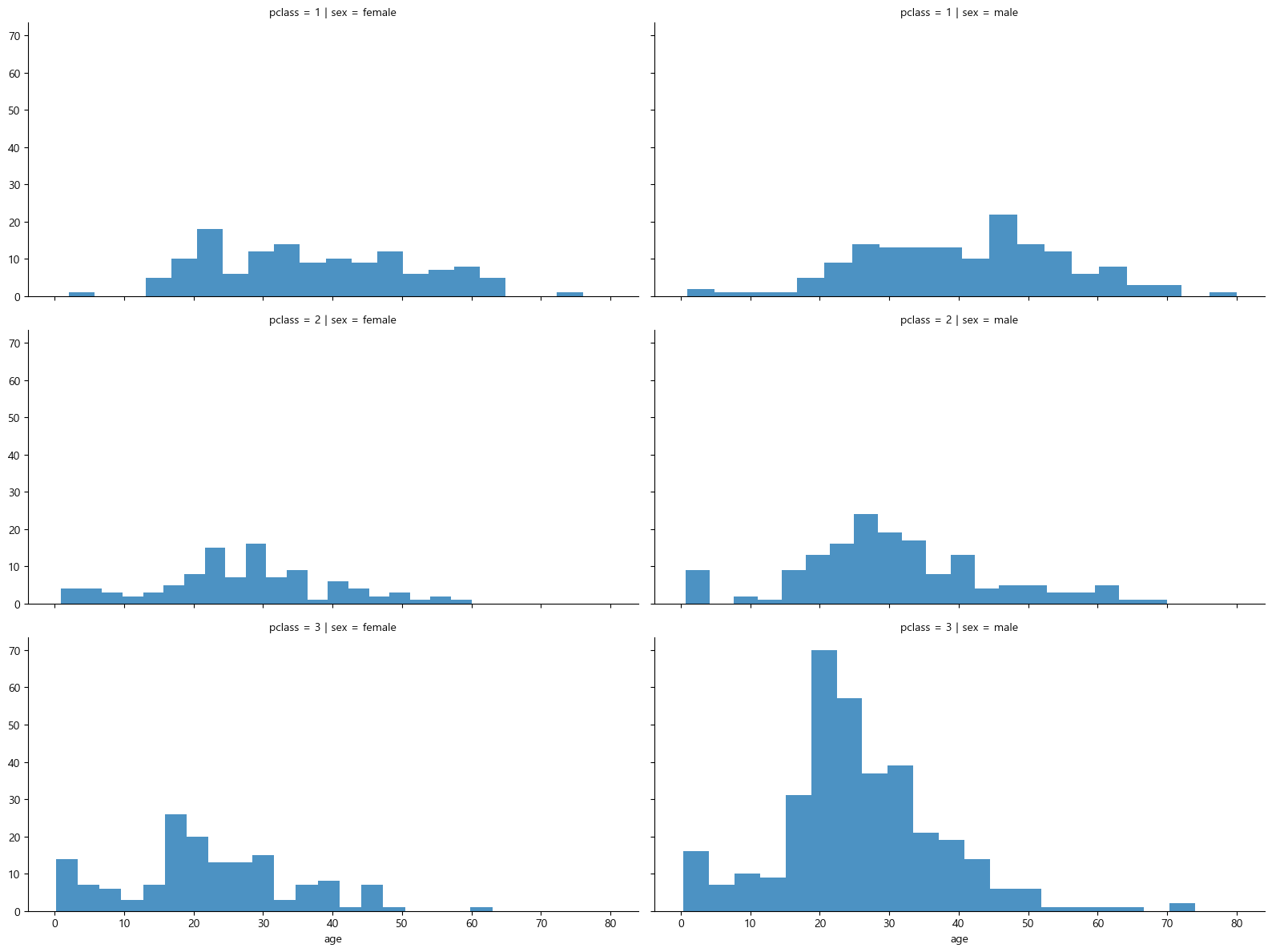
선실등급과 성별에 따른 나이분포 데이터 확인결과
- 3등실에 가장 많은 인원이 탑승하고 있었다
- 3등실에 많은 남성이 타고 있었다(특히, 20대)
-> 3등실의 사망율이 높아서 남성의 사망율이 높게 집계된 가능성이 있다.
-> 남성의 사망율이 높아서 3등실의 사망율이 높게 집계된 가능성이 있다.
-> 아직 인과관계는 알 수 없다
나이분포 데이터
# 나이분포 데이터
import plotly.express as px

fig = px.histogram(titanic, x="age")
fig.show()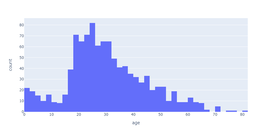
나이분포 데이터 확인결과
- 탑승객의 대다수는 20,30대이다
- 그 중 20대 인원이 가장 많다
선실 등급별 생존율
# 선실 등급별 생존율
grid = sns.FacetGrid(titanic, row='pclass', col='survived', height=4, aspect=2)
grid.map(plt.hist, 'age', alpha=0.5, bins=20)
grid.add_legend()
plt.show()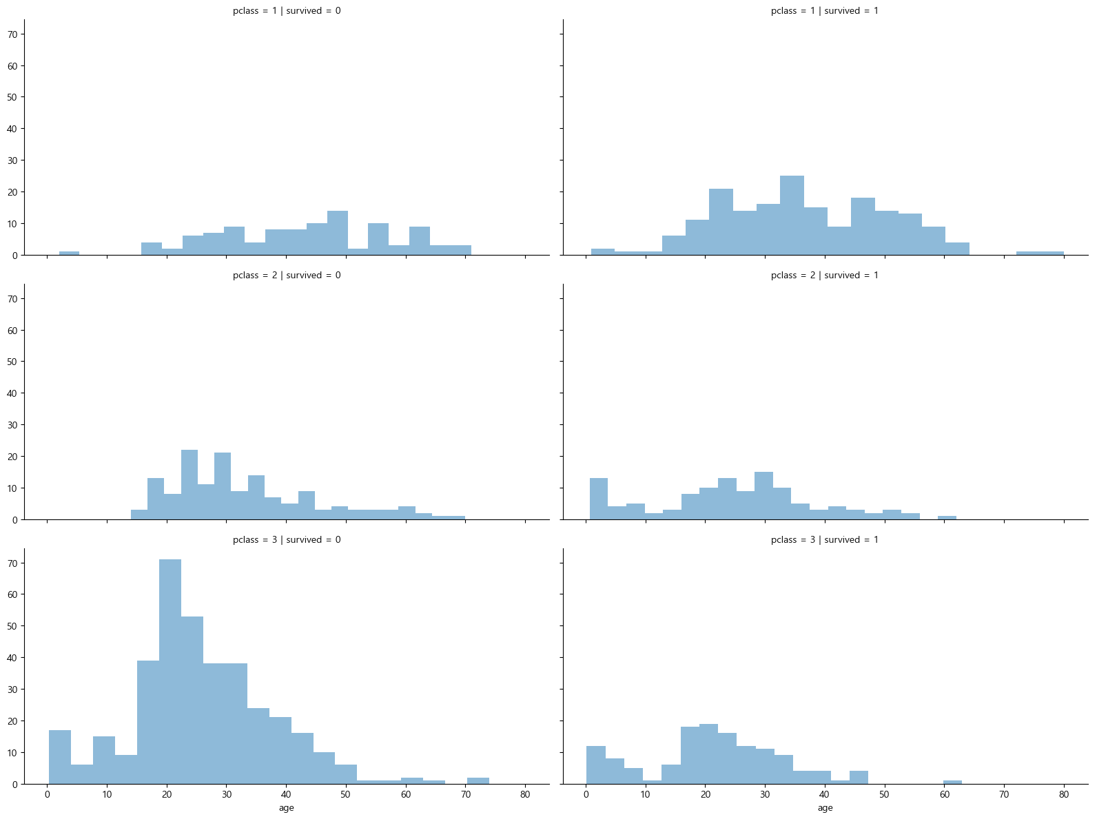
선실 등급별 생존율 확인결과
- 선실등급이 높을수록 생존율이 높다
나이 -> 연령층
# pd.cut() : 특정 칼럼을 특정기준으로 분할해서 재정의
titanic['age_cat'] = pd.cut(titanic['age'], bins=[0,7,15,30,60,100], include_lowest=True, labels=['baby','teen','young','adult','old'])
titanic.head()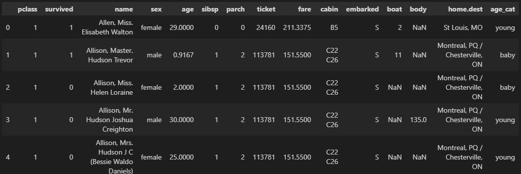
선실, 연령, 성별에 따른 생존데이터
# 선실, 연령, 성별에 따른 생존 데이터
plt.figure(figsize=(12,4))

plt.subplot(131)
sns.barplot(data=titanic, x='pclass', y='survived')

plt.subplot(132)
sns.barplot(data=titanic, x='age_cat', y='survived')

plt.subplot(133)
sns.barplot(data=titanic, x='sex', y='survived')

plt.subplots_adjust(top=1, bottom=0.1, left=0.1, right=1, hspace=0.5, wspace=0.5)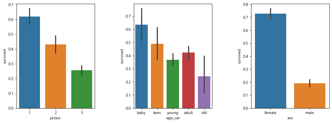
선실, 연령, 성별에 따른 생존데이터 확인결과
- 선실등급이 높을수록 생존율이 높음
- 나이 어릴수록 생존율이 높음
- 여성의 생존율이 높음
성별 생존율 데이터
fig, axes = plt.subplots(nrows=1, ncols=2, figsize=(14,6))
women = titanic[titanic['sex']=='female']
men = titanic[titanic['sex']=='male']

ax = sns.histplot(data=women[women['survived']==1]['age'], bins=20, label='survived', ax=axes[0], kde=False)
ax = sns.histplot(data=women[women['survived']==0]['age'], bins=40, label='not survived', ax=axes[0], kde=False)
ax.legend(); ax.set_title("Female")

ax = sns.histplot(data=men[men['survived']==1]['age'], bins=20, label='survived', ax=axes[1], kde=False)
ax = sns.histplot(data=men[men['survived']==0]['age'], bins=40, label='not survived', ax=axes[1], kde=False)
ax.legend(); ax.set_title("Male")
plt.show()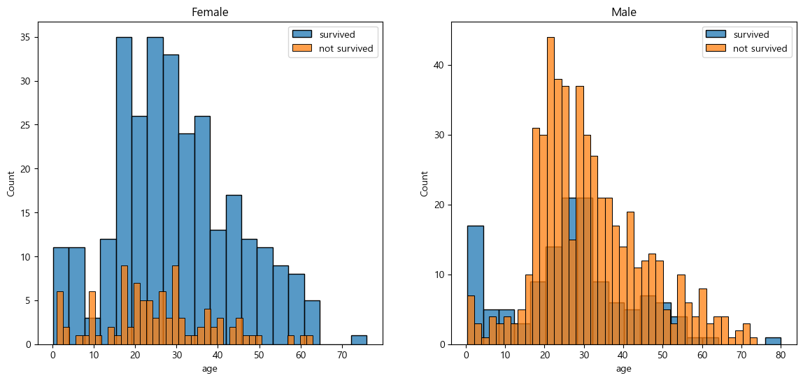
성별 생존율 데이터
- 여성의 생존율이 높음
- 남성의 생존율이 낮음
사회적 신분 데이터
# 사회적 신분 데이터 생성
import re

title = []
for idx, dataset in titanic.iterrows():
    tmp = dataset['name']
    title.append(re.search('\,\s\w+(\s\w+)?\.',tmp).group()[2:-1])

titanic['title']=title
titanic.head()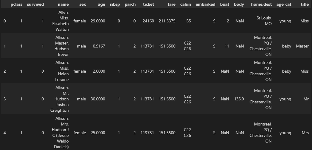
pd.crosstab(titanic['title'], titanic['sex'])
----------------------------------------------
sex           female  male
title
Capt               0     1
Col                0     4
Don                0     1
Dona               1     0
Dr                 1     7
Jonkheer           0     1
Lady               1     0
Major              0     2
Master             0    61
Miss             260     0
Mlle               2     0
Mme                1     0
Mr                 0   757
Mrs              197     0
Ms                 2     0
Rev                0     8
Sir                0     1
the Countess       1     0
귀족명칭 변경
# 귀족의 명칭이 다양하므로 귀족여성과 귀족남성으로 분류한다
# Dr에 여성이 1명 존재하는데, 편의성 남성으로 분류한다

# 평민
titanic['title'] = titanic['title'].replace('Mlle','Miss')
titanic['title'] = titanic['title'].replace('Ms','Miss')
titanic['title'] = titanic['title'].replace('Mme','Mrs')

# 귀족
Rare_f = ['Dona','Lady','the Countess']
Rare_m = ['Dr','Capt','Col','Don','Jonkheer','Major','Master','Rev','Sir']

for each in Rare_f:
    titanic['title'] = titanic['title'].replace(each, 'Rare_f')

for each in Rare_m:
    titanic['title'] = titanic['title'].replace(each, 'Rare_m')

titanic['title'].unique()
----------------------------------------------------------------------------
array(['Miss', 'Rare_m', 'Mr', 'Mrs', 'Rare_f'], dtype=object)titanic[['title', 'survived']].groupby(['title'], as_index=False).mean().sort_values(by='survived')
---------------------------------------------------
title survived
1 Mr 0.162483
4 Rare_m 0.448276
0 Miss 0.678030
2 Mrs 0.787879
3 Rare_f 1.000000사회적 신분 생존율 확인 결과
- 생존율
- 평민남성 -> 귀족남성 -> 평민여성 -> 귀족여성
3) 타이타닉의 생존진실
1912년 4월 14일 밤 11시 40분,에 빙산을 육안으로 발견했다. 이 당시 빙산의 10분의9는 숨어있었기 때문에 빙산을 발견했을 때는 이미 늦은 뒤였다.
4월 15일 0시 15분, 인근선박에 구조요청을 했다. 20km 정도의 거리에 화물선 캘리포니안호가 있었지만 1명밖에 없는 통신사가 피로누적으로 취침 중이라 연락을 받지 못했다.
이 일 이후 교대근무를 통해 통신사가 항상 대기하도록하는 국제규약이 생겨났다.

90km 밖에 있던 구조대가 도착한 시간은 오전 4시로, 타이타닉이 완전히 침몰하고 1시간 40분 뒤에 도착했다.


당시 2등 항해사 라이틀러는 선장에게 여자와 어린이를 먼저 태울 것을 건의하고 선장이 승인했다.

-> 여성과 아이들의 생존비율이 높은 이유
4) DecisionTree 활용
전처리
- 문자 -> 숫자
- 결측치 제외
titanic.info()
# age에 263개, fare에 1개의 결측치를 확인
---------------------------------------------------
<class 'pandas.core.frame.DataFrame'>
RangeIndex: 1309 entries, 0 to 1308
Data columns (total 16 columns):
 #   Column     Non-Null Count  Dtype
---  ------     --------------  -----
 0   pclass     1309 non-null   int64
 1   survived   1309 non-null   int64
 2   name       1309 non-null   object
 3   sex        1309 non-null   object
 4   age        1046 non-null   float64
 5   sibsp      1309 non-null   int64
 6   parch      1309 non-null   int64
 7   ticket     1309 non-null   object
 8   fare       1308 non-null   float64
 9   cabin      295 non-null    object
 10  embarked   1307 non-null   object
 11  boat       486 non-null    object
 12  body       121 non-null    float64
 13  home.dest  745 non-null    object
 14  age_cat    1046 non-null   category
 15  title      1309 non-null   object
dtypes: category(1), float64(3), int64(4), object(8)
memory usage: 155.0+ KB
LabelEncoder
-
문자를 숫자로, 숫자를 문자로 변환
-
머신러닝에 적용하기 위해서는 문자를 숫자로 변환 필요
-
학습이 끝난 후 얻은 결과를 숫자로 변환해서 확인 가능
# 예시용 데이터프레임 생성
import pandas as pd
df = pd.DataFrame({
    'A' : ['a','b','c','a','b'],
    'B' : [1,2,3,1,0]
})
df
---------------------------------
   A  B
0  a  1
1  b  2
2  c  3
3  a  1
4  b  0
# 데이터를 LabelEncoder에 fit
from sklearn.preprocessing import LabelEncoder
le = LabelEncoder()
le.fit(df['A'])
le.classes_
-------------------------------------------------
array(['a', 'b', 'c'], dtype=object)# 문자->숫자
df['le_A'] = le.transform(df['A'])
df
-------------------------------------------------
A B le_A
0 a 1 0
1 b 2 1
2 c 3 2
3 a 1 0
4 b 0 1# 한번에 fit과 변환
le.fit_transform(df['A'])
--------------------------
array([0, 1, 2, 0, 1])# 숫자->문자
le.inverse_transform(df['le_A'])
---------------------------------
array(['a', 'b', 'c', 'a', 'b'], dtype=object)
# 문자를 숫자로 변환
from sklearn.preprocessing import LabelEncoder

le = LabelEncoder()
le.fit(titanic['sex'])
titanic['gender'] = le.transform(titanic['sex'])
titanic.head()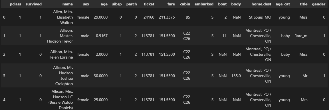
# 결측치 처리
titanic = titanic[titanic['age'].notnull()]
titanic = titanic[titanic['fare'].notnull()]
titanic.info()
----------------------------------------------------------------
<class 'pandas.core.frame.DataFrame'>
Int64Index: 1045 entries, 0 to 1308
Data columns (total 17 columns):
 #   Column     Non-Null Count  Dtype
---  ------     --------------  -----
 0   pclass     1045 non-null   int64
 1   survived   1045 non-null   int64
 2   name       1045 non-null   object
 3   sex        1045 non-null   object
 4   age        1045 non-null   float64
 5   sibsp      1045 non-null   int64
 6   parch      1045 non-null   int64
 7   ticket     1045 non-null   object
 8   fare       1045 non-null   float64
 9   cabin      272 non-null    object
 10  embarked   1043 non-null   object
 11  boat       417 non-null    object
 12  body       119 non-null    float64
 13  home.dest  685 non-null    object
 14  age_cat    1045 non-null   category
 15  title      1045 non-null   object
 16  gender     1045 non-null   int32
dtypes: category(1), float64(3), int32(1), int64(4), object(8)
memory usage: 135.9+ KB
상관관계 확인
correlation_matrix = titanic.corr().round(1)
plt.figure(figsize=(7,7))
sns.heatmap(data=correlation_matrix, annot=True, cmap='bwr')
plt.show()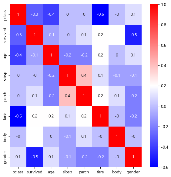
모델학습
from sklearn.model_selection import train_test_split

# 낮은상관관계인 body를 제외한 나머지를 특성데이터로 선정
X = titanic[['pclass','age', 'sibsp', 'parch','fare','gender']]
y = titanic['survived']

X_train, X_test, y_train, y_test = train_test_split(X, y, test_size=0.2, random_state=13)
학습결과 평가
from sklearn.tree import DecisionTreeClassifier
from sklearn.metrics import accuracy_score

dt = DecisionTreeClassifier(max_depth=4, random_state=13)
dt.fit(X_train, y_train)

pred = dt.predict(X_test)
print(accuracy_score(y_test, pred))
-------------------------------------------------------------------
0.7655502392344498
5) 주인공 생존율 예측
디카프리오 생존율 예측
# 디카프리오의 생존율예측

import numpy as np

# 'pclass','age', 'sibsp', 'parch','fare','gender'
dicaprio = np.array([[3, 18, 0, 0, 5, 1]])
print('Decaprio : ', dt.predict_proba(dicaprio)[0, 1])
-------------------------------------------------------
Decaprio :  0.16728624535315986
위즐렛 생존율 예측
# 윈슬릿의 생존율 예측
winslet = np.array([[1, 16, 1, 1, 100, 0]])
print('Winslet : ', dt.predict_proba(winslet)[0, 1])
-------------------------------------------------------
Winslet :  1.0
주인공 생존율 예측 결과
- 디카프리오
6) 추가 작업
중요 칼럼 비율확인
titanic_clf_model = dict(zip(['pclass','age', 'sibsp', 'parch','fare','gender'], dt.feature_importances_))
titanic_clf_model
-----------------------------------------------------------------------------------------------------------
{'pclass': 0.21810410579663048,
 'age': 0.08967670576280189,
 'sibsp': 0.006825017286167317,
 'parch': 0.0,
 'fare': 0.06730002830718068,
'gender': 0.6180941428472196}- 'parch'와 'sibsp', 'fare'은 중요하지 않다.
- 'gender'와 'pclass'는 중요 칼럼이다.
'gender'와 'pclass'만 사용한 모델링
from sklearn.model_selection import train_test_split

# 중요한 2개의 칼럼만 사용
X = titanic[['pclass', 'gender']]
y = titanic['survived']

X_train, X_test, y_train, y_test = train_test_split(X, y, test_size=0.2, random_state=13)
from sklearn.tree import DecisionTreeClassifier
from sklearn.metrics import accuracy_score
dt = DecisionTreeClassifier(max_depth=4, random_state=13)
dt.fit(X_train, y_train)
pred = dt.predict(X_test)
print(accuracy_score(y_test, pred))
-----------------------------------------------------------
0.7559808612440191# 디카프리오의 생존율예측
import numpy as np
# 'pclass','age', 'sibsp', 'parch','fare','gender'
dicaprio = np.array([[3, 1]])
print('Decaprio : ', dt.predict_proba(dicaprio)[0, 1])
----------------------------------------------------------
Decaprio : 0.17562724014336917# 윈슬릿의 생존율 예측
winslet = np.array([[1, 0]])
print('Winslet : ', dt.predict_proba(winslet)[0, 1])
------------------------------------------------------
Winslet : 0.9727272727272728