해당 글은 제로베이스데이터스쿨 학습자료를 참고하여 작성되었습니다
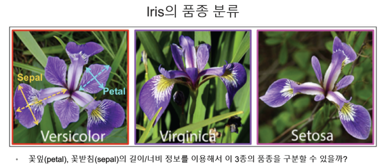
1. Iris 데이터
-
data : 종류를 맞추기 위한 정보(=문제)
-
target : 종류의 인덱스(=정답)
-
target_names : 종류의 명칭
-
DESCR : iris 데이터의 전체 정보
-
feature_names : data의 정보(무엇을 의미하는지)
1) 칼럼확인
from sklearn.datasets import load_iris

iris = load_iris()
iris.keys()
-----------------------------------------------------------------------------------------------------------
dict_keys(['data', 'target', 'frame', 'target_names', 'DESCR', 'feature_names', 'filename', 'data_module'])
데이터확인
print(iris["data"])
----------------------------------
[[5.1 3.5 1.4 0.2]
 [4.9 3.  1.4 0.2]
 [4.7 3.2 1.3 0.2]
...
 [6.3 2.5 5.  1.9]
 [6.5 3.  5.2 2. ]
 [6.2 3.4 5.4 2.3]
 [5.9 3.  5.1 1.8]]
타겟확인
print(iris["target"])
--------------------------------------------------------------------------
[0 0 0 0 0 0 0 0 0 0 0 0 0 0 0 0 0 0 0 0 0 0 0 0 0 0 0 0 0 0 0 0 0 0 0 0 0
 0 0 0 0 0 0 0 0 0 0 0 0 0 1 1 1 1 1 1 1 1 1 1 1 1 1 1 1 1 1 1 1 1 1 1 1 1
 1 1 1 1 1 1 1 1 1 1 1 1 1 1 1 1 1 1 1 1 1 1 1 1 1 1 2 2 2 2 2 2 2 2 2 2 2
 2 2 2 2 2 2 2 2 2 2 2 2 2 2 2 2 2 2 2 2 2 2 2 2 2 2 2 2 2 2 2 2 2 2 2 2 2
 2 2]
타겟이름확인
print(iris["target_names"])
------------------------------------
['setosa' 'versicolor' 'virginica']
데이터셋 정보확인
print(iris.get("DESCR"))
--------------------------------
.. _iris_dataset:

Iris plants dataset
--------------------

**Data Set Characteristics:**

    :Number of Instances: 150 (50 in each of three classes)
    :Number of Attributes: 4 numeric, predictive attributes and the class
    :Attribute Information:
        - sepal length in cm
        - sepal width in cm
        - petal length in cm
        - petal width in cm
        - class:
                - Iris-Setosa
                - Iris-Versicolour
                - Iris-Virginica

    :Summary Statistics:

    ============== ==== ==== ======= ===== ====================
                    Min  Max   Mean    SD   Class Correlation
    ============== ==== ==== ======= ===== ====================
    sepal length:   4.3  7.9   5.84   0.83    0.7826
    sepal width:    2.0  4.4   3.05   0.43   -0.4194
    petal length:   1.0  6.9   3.76   1.76    0.9490  (high!)
    petal width:    0.1  2.5   1.20   0.76    0.9565  (high!)
    ============== ==== ==== ======= ===== ====================

    :Missing Attribute Values: None
    :Class Distribution: 33.3% for each of 3 classes.
    :Creator: R.A. Fisher
    :Donor: Michael Marshall (MARSHALL%PLU@io.arc.nasa.gov)
    :Date: July, 1988

The famous Iris database, first used by Sir R.A. Fisher. The dataset is taken
from Fisher's paper. Note that it's the same as in R, but not as in the UCI
Machine Learning Repository, which has two wrong data points.

This is perhaps the best known database to be found in the
pattern recognition literature.  Fisher's paper is a classic in the field and
is referenced frequently to this day.  (See Duda & Hart, for example.)  The
data set contains 3 classes of 50 instances each, where each class refers to a
type of iris plant.  One class is linearly separable from the other 2; the
latter are NOT linearly separable from each other.

.. topic:: References

   - Fisher, R.A. "The use of multiple measurements in taxonomic problems"
     Annual Eugenics, 7, Part II, 179-188 (1936); also in "Contributions to
     Mathematical Statistics" (John Wiley, NY, 1950).
   - Duda, R.O., & Hart, P.E. (1973) Pattern Classification and Scene Analysis.
     (Q327.D83) John Wiley & Sons.  ISBN 0-471-22361-1.  See page 218.
   - Dasarathy, B.V. (1980) "Nosing Around the Neighborhood: A New System
     Structure and Classification Rule for Recognition in Partially Exposed
     Environments".  IEEE Transactions on Pattern Analysis and Machine
     Intelligence, Vol. PAMI-2, No. 1, 67-71.
   - Gates, G.W. (1972) "The Reduced Nearest Neighbor Rule".  IEEE Transactions
     on Information Theory, May 1972, 431-433.
   - See also: 1988 MLC Proceedings, 54-64.  Cheeseman et al"s AUTOCLASS II
     conceptual clustering system finds 3 classes in the data.
   - Many, many more ...
특성이름확인
print(iris.get("feature_names"))
----------------------------------------------------------------------------------
['sepal length (cm)', 'sepal width (cm)', 'petal length (cm)', 'petal width (cm)']
2) 데이터 이해하기
데이터프레임 생성
import pandas as pd

iris_pd = pd.DataFrame(iris.data, columns=iris.feature_names)
iris_pd
------------------------------------------------------------------------------
     sepal length (cm)  sepal width (cm)  petal length (cm)  petal width (cm)
0                  5.1               3.5                1.4               0.2
1                  4.9               3.0                1.4               0.2
2                  4.7               3.2                1.3               0.2
3                  4.6               3.1                1.5               0.2
4                  5.0               3.6                1.4               0.2
..                 ...               ...                ...               ...
145                6.7               3.0                5.2               2.3
146                6.3               2.5                5.0               1.9
147                6.5               3.0                5.2               2.0
148                6.2               3.4                5.4               2.3
149                5.9               3.0                5.1               1.8
타겟 추가
iris_pd['species'] = iris.target
iris_pd.head()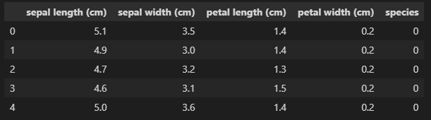
이해를 위한 시각화
각 칼럼과 데이터 간의 관계확인
import matplotlib.pyplot as plt
import seaborn as sns
from matplotlib.pyplot import rc

rc('font', family='Malgun Gothic')

plt.figure(figsize=(12,12))
plt.subplot(2, 2, 1)
sns.boxplot(data=iris_pd, x='sepal length (cm)', y='species', orient='h');
plt.title('꽃받침 길이')

plt.subplot(2, 2, 2)
sns.boxplot(data=iris_pd, x='sepal width (cm)', y='species', orient='h');
plt.title('꽃받침 너비')

plt.subplot(2, 2, 3)
sns.boxplot(data=iris_pd, x='petal length (cm)', y='species', orient='h');
plt.title('꽃잎 길이')

plt.subplot(2, 2, 4)
sns.boxplot(data=iris_pd, x='petal width (cm)', y='species', orient='h');
plt.title('꽃잎 너비')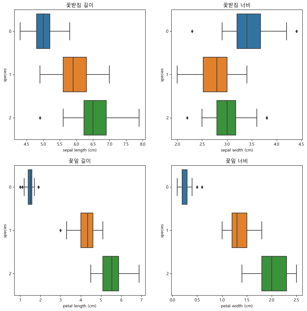
칼럼별 상관관계 시각화
sns.pairplot(data=iris_pd, hue='species');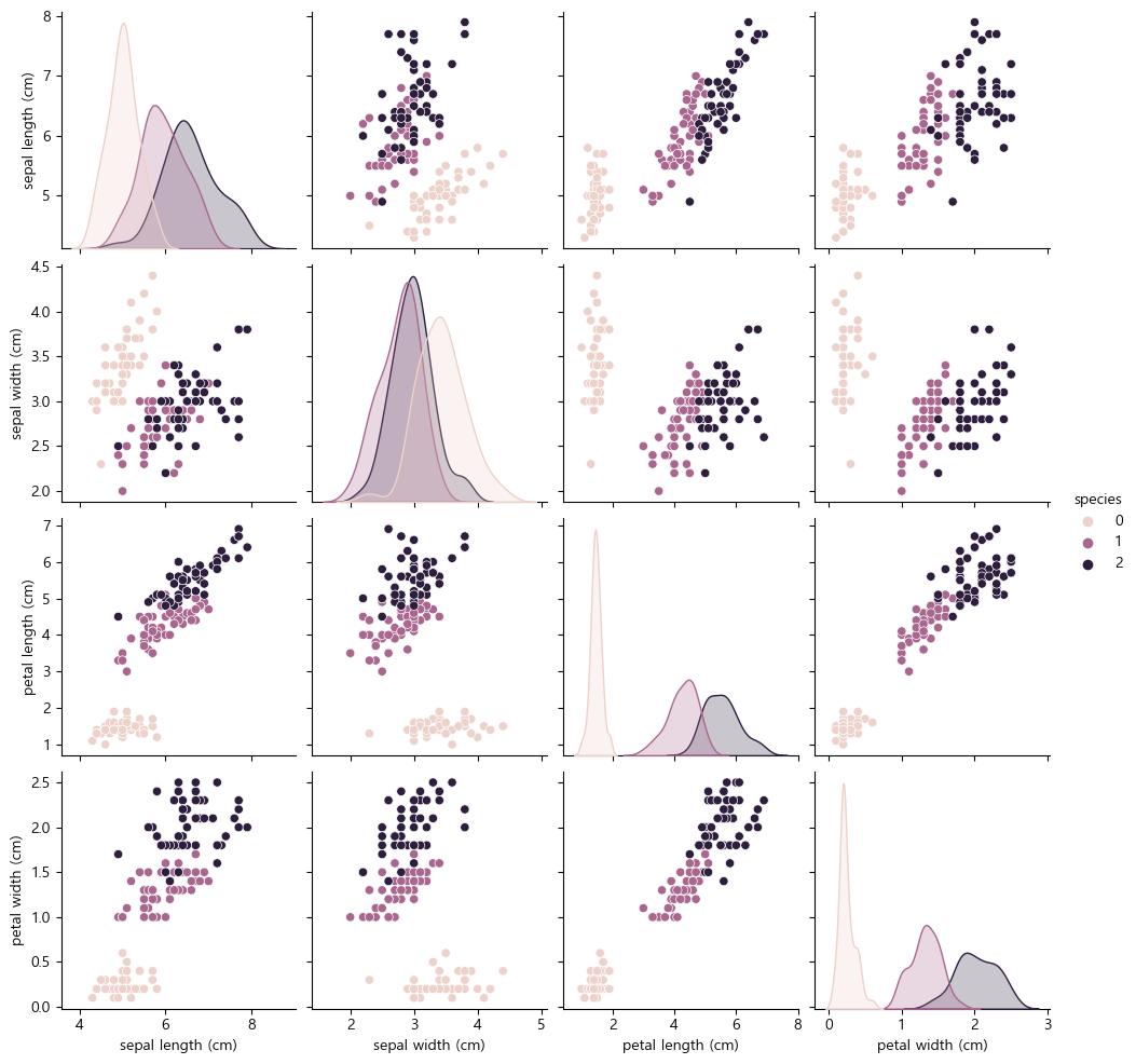
유효한 칼럼관계 상세 확인
sns.pairplot(data=iris_pd, vars=['petal length (cm)', 'petal width (cm)'], hue='species', height=4);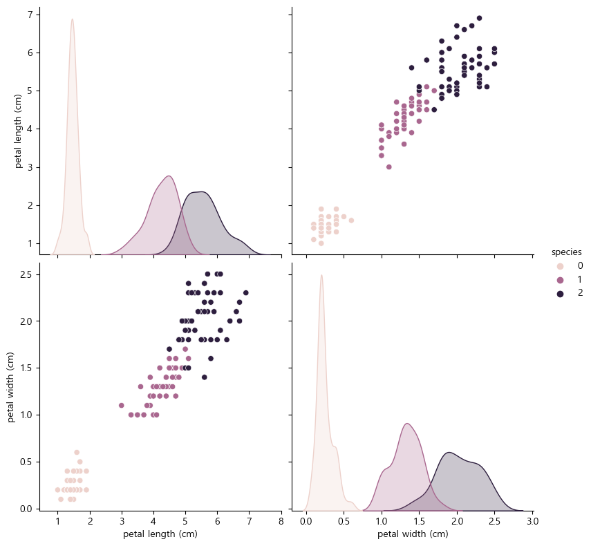
scatter 시각화
plt.figure(figsize=(12,6))
sns.scatterplot(data=iris_pd, x='petal length (cm)', y='petal width (cm)', hue='species', palette='Set2');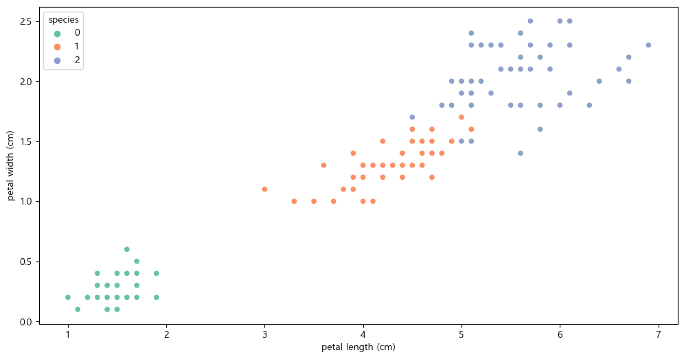
setosa를 배제한 scatter 시각화
iris_12 = iris_pd[iris_pd['species']!=0]
sns.scatterplot(data=iris_12, x='petal length (cm)', y='petal width (cm)', hue='species', palette='Set2');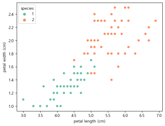
3)분석내용
분류 방법에 대한 분석
- setosa : petal(꽃잎)의 length&width 가 작은 것
- versicolor : petal length & width가 특정 값을 기준으로 작은 것
- virginica : petal length & width가 특정 값을 기준으로 큰 것
분류에 관한 데이터 이해
- sepal(꽃받침)은 petal에 비해 낮은 분류 성능을 가지고 있다
- petal만 사용해서 분류가 가능할 것으로 보인다
- 데이터가 일부 겹쳐있지만 특정 값을 기준으로 분류한다면 대부분 정답이다
기준 값은 어떻게 결정할 것인가???
-
사람의 추측, 눈대중으로 결정할 수 도 있지만 과연 최선인가??
-
최적의 기준(계수)을 결정하기 위해 사용하는 것이 알고리즘, 머신러닝 등 이다.
-
수치적인 기준이 있다면 객관적인 이해가 가능하다.
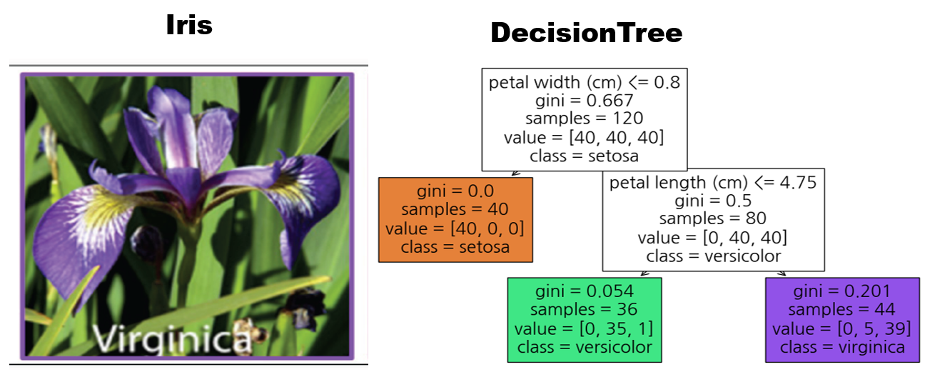
2. Decision Tree
- 직관적인 분류방식(True or False)
- 단순하고 효과적인 방식
- 앙상블 계열의 기초
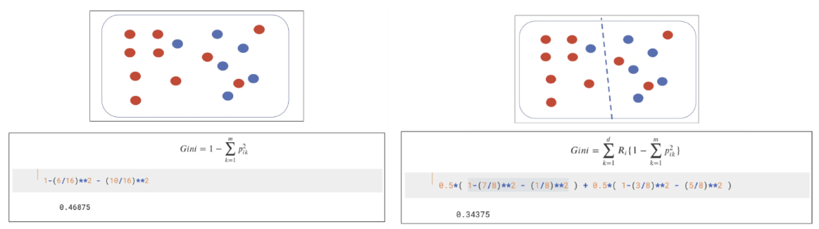
1) Decision Tree의 분할 기준
- 엔트로피
- 지니계수
- 두 기준은 낮을수록 좋음
엔트로피(entropy)
-
열역학의 용어로 물질의 열적 상태를 나타내는 물리량
-
무질서도, 불확실성을 의미함
-

지니 계수(Gini index)
-
불순도율을 의미함
-
엔트로피와 동일하게 수치가 낮을수록 좋은 결과를 얻음
-
log를 사용하는 엔트로피와 다르게 지니계수는 단순 산술이므로 처리부하가 적음
-
2) DecionsTree 학습과 평가
학습
from sklearn.tree import DecisionTreeClassifier

iris_tree = DecisionTreeClassifier()
feature = iris.data[:, 2:] # 학습데이터(petal만 사용)
target = iris.target       # 정답 데이터
iris_tree.fit(feature, target)
결과 확인
# 학습 결과 확인
from sklearn.metrics import accuracy_score

y_pred_tr = iris_tree.predict(feature)
y_pred_tr
-----------------------------------------------------------------------
array([0, 0, 0, 0, 0, 0, 0, 0, 0, 0, 0, 0, 0, 0, 0, 0, 0, 0, 0, 0, 0, 0,
       0, 0, 0, 0, 0, 0, 0, 0, 0, 0, 0, 0, 0, 0, 0, 0, 0, 0, 0, 0, 0, 0,
       0, 0, 0, 0, 0, 0, 1, 1, 1, 1, 1, 1, 1, 1, 1, 1, 1, 1, 1, 1, 1, 1,
       1, 1, 1, 1, 2, 1, 1, 1, 1, 1, 1, 1, 1, 1, 1, 1, 1, 1, 1, 1, 1, 1,
       1, 1, 1, 1, 1, 1, 1, 1, 1, 1, 1, 1, 2, 2, 2, 2, 2, 2, 2, 2, 2, 2,
       2, 2, 2, 2, 2, 2, 2, 2, 2, 2, 2, 2, 2, 2, 2, 2, 2, 2, 2, 2, 2, 2,
2, 2, 2, 2, 2, 2, 2, 2, 2, 2, 2, 2, 2, 2, 2, 2, 2, 2])iris.target
------------------------------------------------------------------------
array([0, 0, 0, 0, 0, 0, 0, 0, 0, 0, 0, 0, 0, 0, 0, 0, 0, 0, 0, 0, 0, 0,
0, 0, 0, 0, 0, 0, 0, 0, 0, 0, 0, 0, 0, 0, 0, 0, 0, 0, 0, 0, 0, 0,
0, 0, 0, 0, 0, 0, 1, 1, 1, 1, 1, 1, 1, 1, 1, 1, 1, 1, 1, 1, 1, 1,
1, 1, 1, 1, 1, 1, 1, 1, 1, 1, 1, 1, 1, 1, 1, 1, 1, 1, 1, 1, 1, 1,
1, 1, 1, 1, 1, 1, 1, 1, 1, 1, 1, 1, 2, 2, 2, 2, 2, 2, 2, 2, 2, 2,
2, 2, 2, 2, 2, 2, 2, 2, 2, 2, 2, 2, 2, 2, 2, 2, 2, 2, 2, 2, 2, 2,
2, 2, 2, 2, 2, 2, 2, 2, 2, 2, 2, 2, 2, 2, 2, 2, 2, 2])정확도 평가
accuracy_score(iris.target, y_pred_tr)
---------------------------------------
0.9933333333333333
DecionsTree 시각화
from sklearn.tree import plot_tree

plt.figure(figsize=(10,10))
plot_tree(iris_tree, filled=True)
plt.show()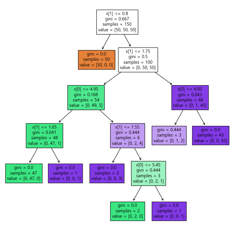
3) 과적합(Overfitting)
- 학습데이터에 과도하게 적합하게 되어 다른 데이터의 정답률(예측)이 감소하는 것
결정 경계
from mlxtend.plotting import plot_decision_regions
import matplotlib

matplotlib.rcParams['axes.unicode_minus'] = False
plt.figure(figsize=(14,8))
plot_decision_regions(X=feature, y=target, clf=iris_tree, legend=2)
plt.title('결정 경계')
plt.show()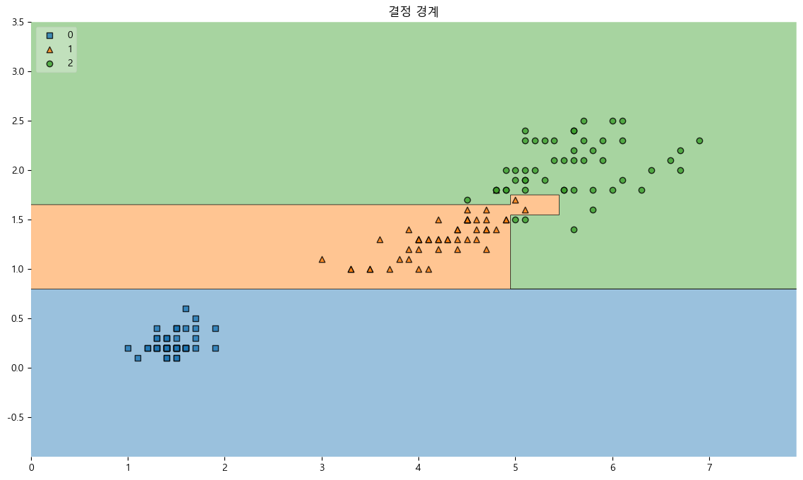
-
1,2번 사이의 경계선이 복잡하고, 위에서 정확도를 구했을 때, 99%가 나왔는데 이것은 과적합된 것이다.
-
주어진 학습데이터 150개에 대해서만 결과가 다음과 같이 나온 것이지, 이것이 모든 iris를 대표한다고 할 수 없기 때문이다.
->성급한 일반화의 오류 가능성 -
복잡한 경계면은 모델의 성능을 결국 나쁘게 만든다.
-
경계면에 복잡한 부근에 있는 데이터들이 이상치일 가능성은 없는것인가? 신뢰할 수 있는가?
-
일반적인 데이터를 기준으로 모델의 성능을 향상시키려면 어느 정도의 오류는 감수해야 한다.
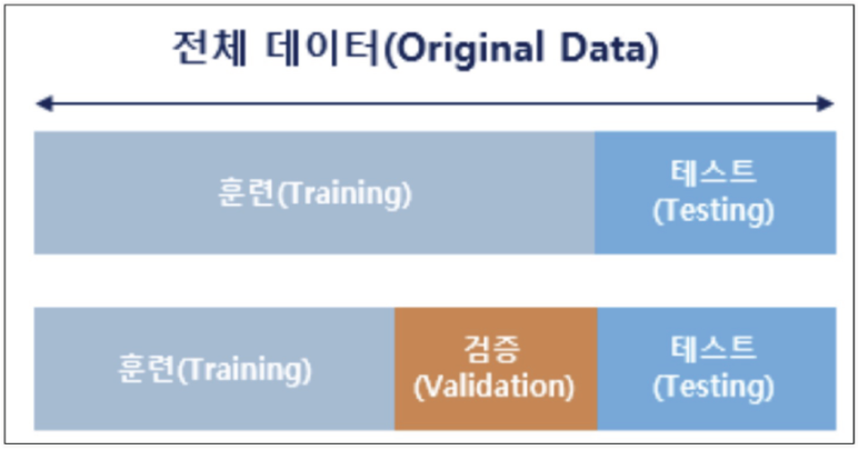
4) 데이터분리
- 데이터를 학습데이터와 검증데이터, 라벨데이터로 분류
- 검증데이터를 따로 준비하여 과적합 최소화
from sklearn.datasets import load_iris
from sklearn.model_selection import train_test_split
import pandas as pd

iris = load_iris()
features = iris.data[:, 2:]
labels = iris.target
# 데이터분리
X_train, X_test, y_train, y_test = train_test_split(features, labels, test_size=0.2, stratify=labels, random_state=13)
# 분리 형태 확인
X_train.shape, X_test.shape
-----------------------------------------------------------------------------------------------------
((120, 2), (30, 2))
train_test_split() 함수
- 1,2번째 요소 : 특성데이터와 정답데이터
- test_size : test 데이터 크기
- shuffle : 데이터 분할전 섞기
- stratify : 분류데이터 비율 동등
- random_state : 랜덤시드
stratify 적용예시
- 분할된 데이터의 갯수를 같은 비율로 설정함
import numpy as np

np.unique(y_test, return_counts=True)
----------------------------------------------------
(array([0, 1, 2]), array([10, 10, 10], dtype=int64))
shuffle 추가설명
- 고정된 훈련데이터와 평가데이터를 사용하지 않고 셔플하는 기능
5) 학습과 평가
DecisionTree 시각화
from sklearn.tree import DecisionTreeClassifier
from sklearn.tree import plot_tree

iris_tree = DecisionTreeClassifier(max_depth=2, random_state=13)
iris_tree.fit(X_train, y_train)

plt.figure(figsize=(7,7))
plot_tree(iris_tree, filled=True)
plt.show()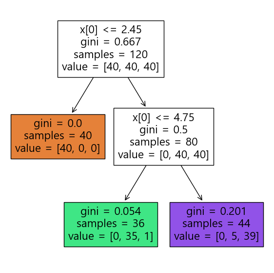
DecisionTreeClassifier() 함수
- criterion : 기준(gini, entropy)
- max_depth : 깊이 설정
- min_samples_split : 노드를 분할하는데 필요한 최소 샘플 수
- min_samples_leaf : 노드에 있어야 하는 최소 샘플 수
- max_features : 최상의 분할을 찾을 때 고려할 최대 기능 수
- random_state : 랜덤시드
- class_weight : 가중치 설정
max_features 추가설명
- 데이터 세트 10개이고 max_features=5인 경우, 의사결정트리를 구성할 때 각 노드에서 임의로 선정한 5개의 데이터 세트를 활용함
평가
from sklearn.metrics import accuracy_score

y_pred_tr = iris_tree.predict(X_train)
accuracy_score(y_train, y_pred_tr)
-------------------------------------------
0.95
결정 경계
학습데이터 결정경계
from mlxtend.plotting import plot_decision_regions
import matplotlib

matplotlib.rcParams['axes.unicode_minus'] = False
plt.figure(figsize=(14,8))
plot_decision_regions(X=X_train, y=y_train, clf=iris_tree, legend=2)
plt.title('결정 경계(train)')
plt.show()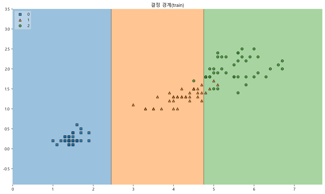
평가데이터 결정경계
plt.figure(figsize=(14,8))
plot_decision_regions(X=X_test, y=y_test, clf=iris_tree, legend=2)
plt.title('결정 경계(test)')
plt.show()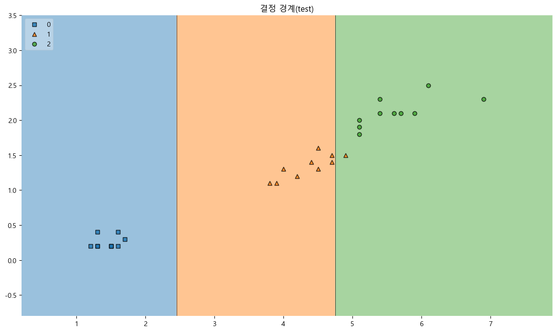
학습&평가 데이터 결정경계
scatter_highlight_kwargs = {'s':150, 'label':'Test data', 'alpha':0.9}
scatter_kwargs = {'s':120, 'edgecolor': None, 'alpha':0.7}

plt.figure(figsize=(12,8))
plot_decision_regions(X=features, y=labels, X_highlight=X_test, clf=iris_tree, legend=2,
                      scatter_highlight_kwargs=scatter_highlight_kwargs,
                      scatter_kwargs=scatter_kwargs,
                      contourf_kwargs={'alpha':0.2})
plt.show()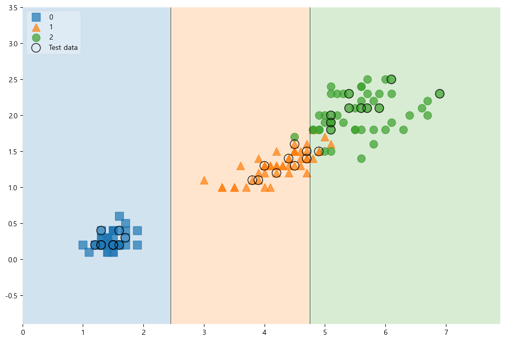
6) 예측
정답 예측
# 예측하기
test_data = [[4.3, 2., 1.2, 1.]]
iris_tree.predict(test_data)
----------------------------------
array([1])iris.target_names[iris_tree.predict(test_data)]
-----------------------------------------------
array(['versicolor'], dtype='<U10')정답 확률 예측
iris_tree.predict_proba(test_data)
---------------------------------------------
array([[0.        , 0.97222222, 0.02777778]])
7) 중요 칼럼 비율
# 중요 칼럼
iris_tree.feature_importances_
--------------------------------------------------------
array([0.        , 0.        , 0.42189781, 0.57810219])
iris_clf_model = dict(zip(iris.feature_names, iris_tree.feature_importances_))
iris_clf_model
-----------------------------------------------
{'sepal length (cm)': 0.0,
'sepal width (cm)': 0.0,
'petal length (cm)': 0.421897810218978,
'petal width (cm)': 0.578102189781022}tuple -> dict
# tuple과 dict
list1 = ['a', 'b', 'c']
list2 = [1,2,3]

dict(zip(list1, list2))
-------------------------
{'a': 1, 'b': 2, 'c': 3}