Normalizing Activations in a Network

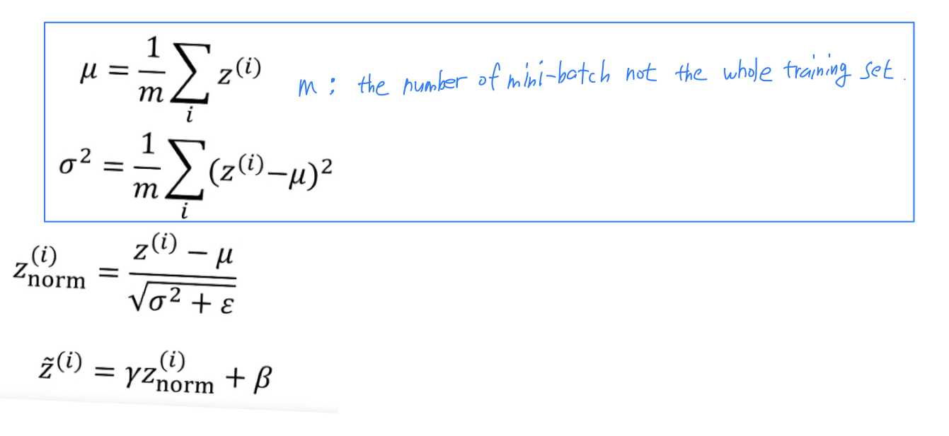
• Batch normalization makes your hyperparameter search problem much easier,
  makes your neural network much more robust(튼튼한).
  And it will also enable you to much more easily train every very deep networks.

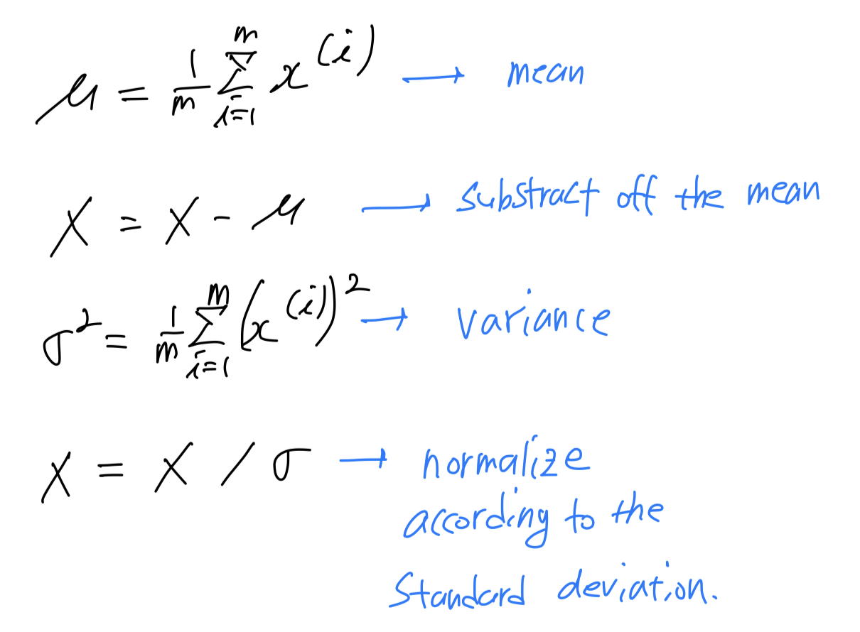
Normalizing inputs to speed up learning.

• Let's see how Batch normalization works.
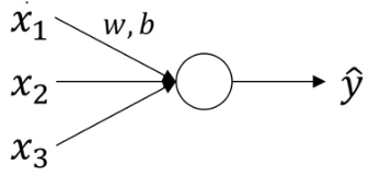
  When training a model, such as logistic regression,
  you might remember that normalizing the input features can speed up learnings
  in compute the means, substract off the means from your training sets, compute the variances, and then normalize your data set according to the variances.
  And we saw in an earlier video how this can turn the contours of you learning problem from something that might be very elongated(길쭉한) something that is more round(둥근),
  and easier for an algorithm like gradient descent to optimize.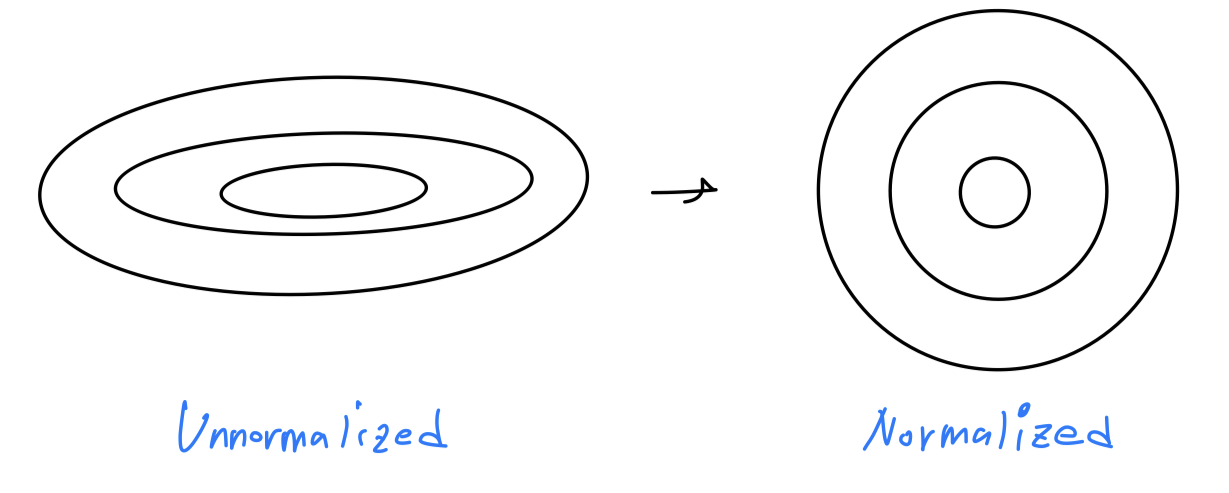So this works,
  in terms of normalizing the input features values to a neural network, alter the logistic regression
  

• In the case of logistic regression,
  we saw how normalizing $X$ maybe helps you train $W, b$ more efficiently.
  
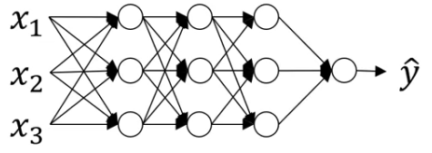
  How about a deeper model?
  You have not just input features $x$, but you have activations $a^{[1]}, a^{[2]}, ...$
  So if you want to train the parameter say $W^{[3]}, b^{[3]}$ would't be nice
  if you can normalize the mean and variance of $a^{[2]}$ to make the training of $W^{[3]}, b^{[3]}$ more efficient?
  So here, the question is, for any hidden layer,
  Can we normalize the values of $a^{[l]}$ so as to train $w^{[l+1]}, b^{[l+1]}$ faster?
  ($a^{[l]}$의 평균과 분산을 normalizing하여 $W^{[l+1]}, b^{[l+1]}$의 training을 더 효율적으로 만들 수 있지 않을까?)
  We will actually normalize values of not $a^{[l]}$ but $z^{[l]}$
  In practice, normalizing $z^{[l]}$ is done much more often.
  ➡️ So this is what batch norm(= batch normalization) does.
  

Implementing Batch Norm

• Given some intermediate values in your Neural Network.
  Let's say that you have some hidden unit values $z^{(1)}$~$z^{(m)}$.
  ($z^{[i](i)}$가 더 정확하지만, 간편하게 하기 위해 몇 번째 layer인지는 생략.)
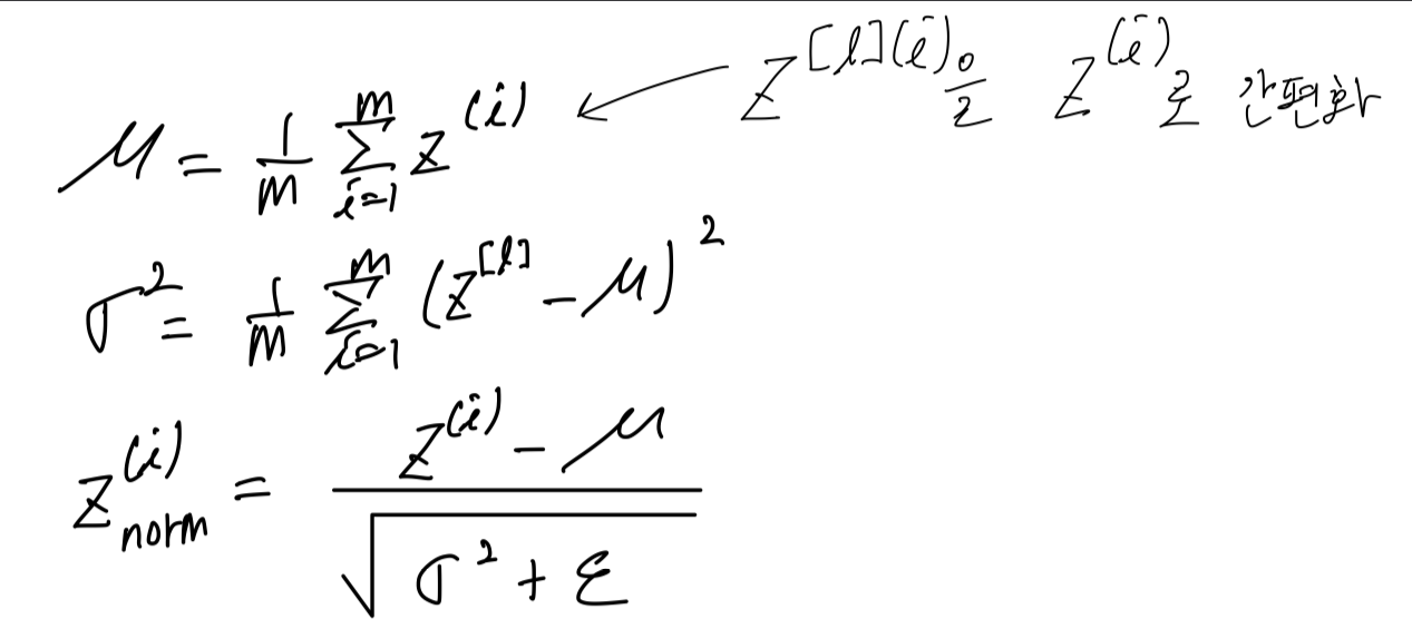  So now every components of $z$ has mean 0 and variance 1.
  But we don't want the hidden units to always have mean 0 and variance 1.
  Maybe it makes sense for hidden units to have different distribution.
  So what we'll do instead is compute $\tilde{\gamma}$.
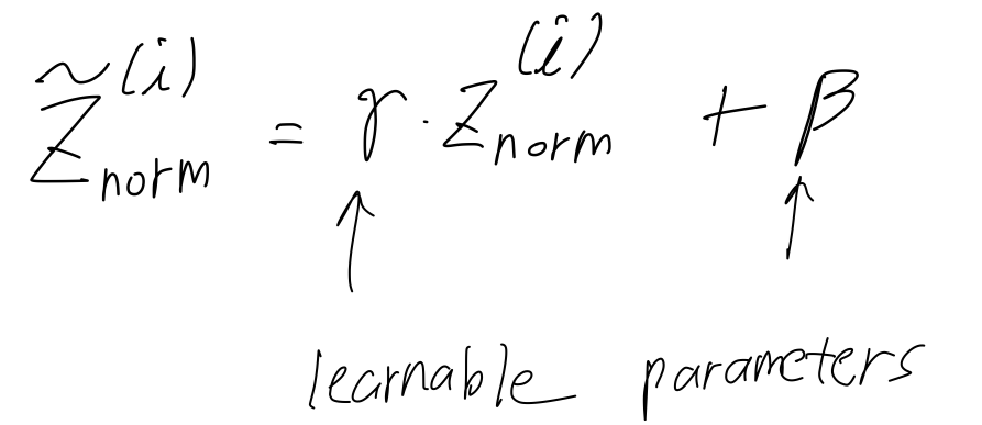  Now, notice that the effect of $\gamma$ and $\beta$ is that
  it allows you to set the mean of $\tilde{z}$ to be whatever you want it to be.
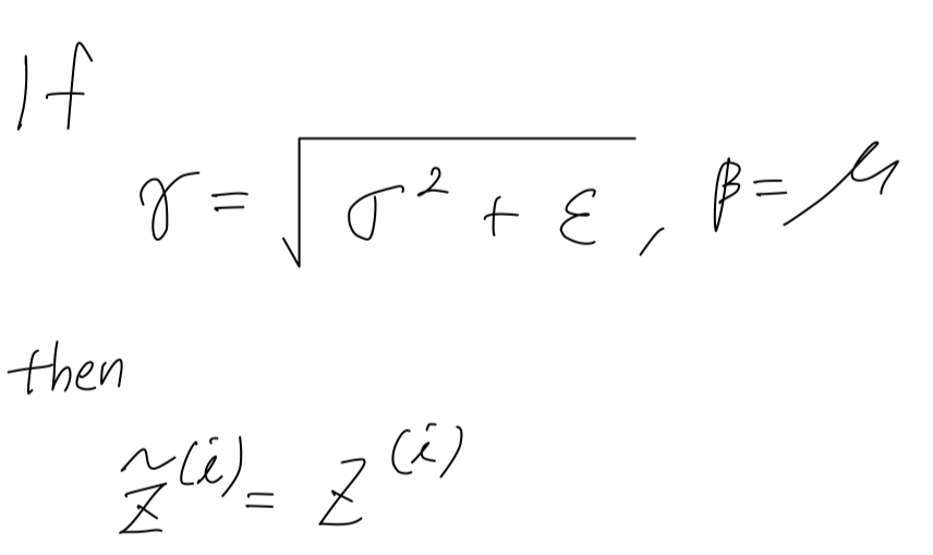  And so by an appropriate setting of the parameters $\gamma, \beta$,
  this normalization step, that is, these four equation is computing essentially the identity function.
  But by choosing other values of $\gamma, \beta$, this allows you to make the hidden unit values have other means and variances as well.
  
  And so the way you fit this into your neural network is,
  whereas previously you were using these values $z^{[1]}, z^{[2]}$ and so on,
  you would now use $\tilde{z}^{[l](i)}$ instead of $z^{[l](i)}$ for the later computation in your neural network.
  
  So the intuition you'll take away from this is that
  we saw how normalizing the input feature $X$ can help learning in a neural network.
  And what batch norm does is it applies that normalization proces not only just to the input layer,
  but also to the values even deep in some hidden layer in the neural network.
  But one difference between the training input and these hidden unit values is
  you might not want your hidden unit values be forced to have mean 0 and variance 1.
  
  For example, if you have a sigmoid function, you don't want your values to always be clustered here.
  You might want them to have a larger variance or have a mean that's different than 0,
  in order to better take advantage of nonlinearlity of the sigmoid function
  rather than have all your values be in just this linear regime.
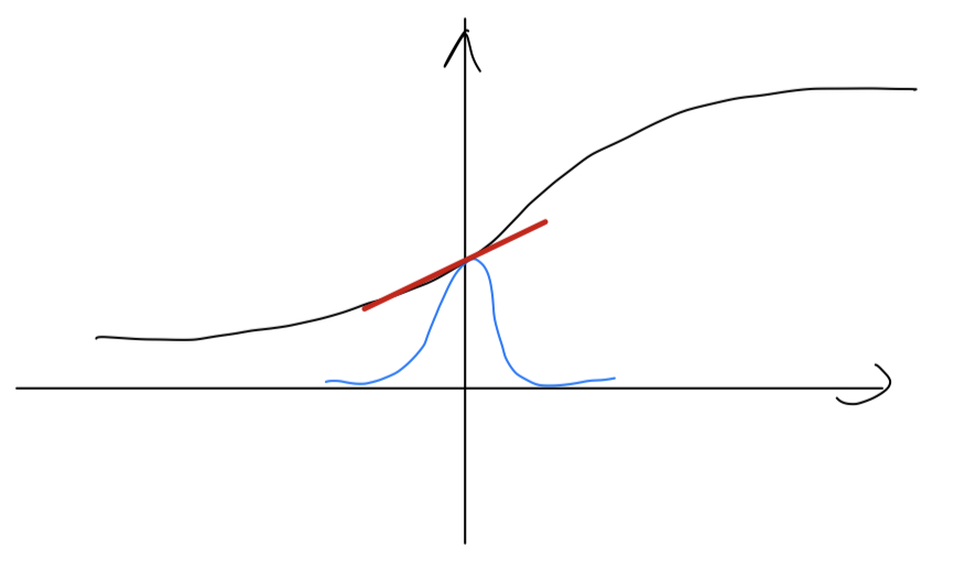  So that's why with the parameters $\gamma, \beta$,
  you can now make sure that your $z^{[l](i)}$ values have the range of values that you want.
  But what it does really is it then shows that your hidden units have standardized mean and variance,
  where the mean and variance are controlled by two explicit parameters $\gamma, \beta$
  which the learning algorithms can set to whatever it wants.
  So what is really does it it normalizes in mean and variance
  of these hidden unit values($z^{[l](i)}$), to have some fixed mean and variance.
  And that mean and variance could be 0 and 1,
  it could be some other value, and it's controlled by these parameters $\gamma, \beta$.

---

Fitting Batch Norm into a Neural Network

• You have seen the equations for how to invent Batch Norm for a single hidden layer.
  Let's see how it fits into the training of a deep network.

Adding Batch Norm to a network

• Let's say you have a neural network like this
  
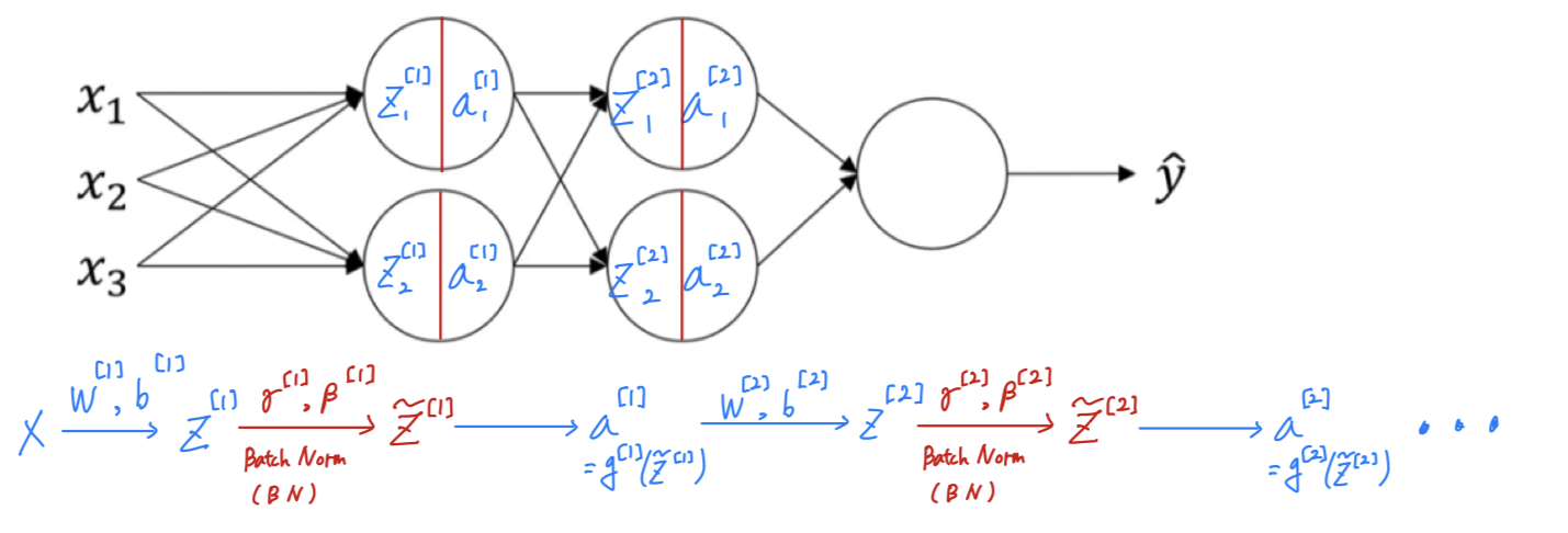
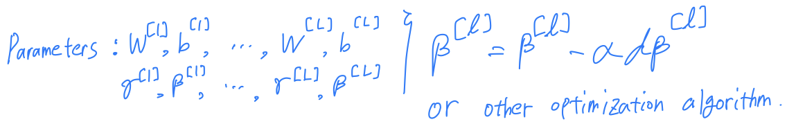
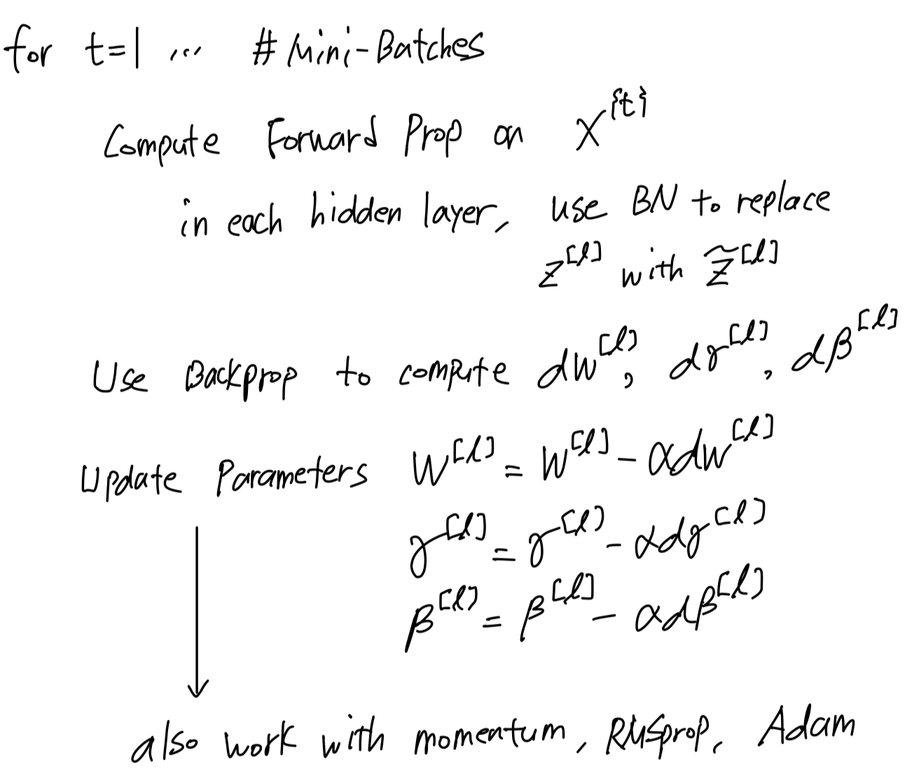
  So now that these are the new parameters of your algorithm.
  You can also use Momentum or RMSprop or Adam in order to update the parameters $\gamma, \beta$
  not just gradient descent.

Working with mini-batches

• In practice, Batch Norm is applied with mini-batches of you training set.
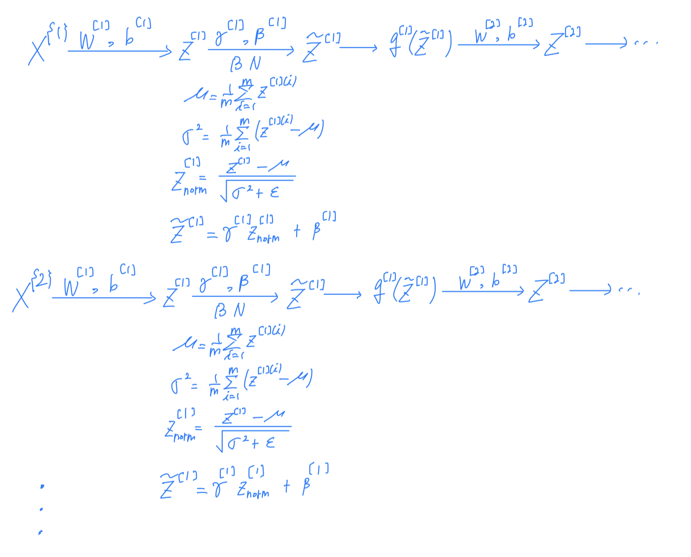  Now, there's one detail to the parameterization that i want to clean up.
  
  Now notice that the way $Z^{[l]}=W^{[l]}a^{[l-1]}+b^{[l]}$.
  What Batch Norm does is
  it is going to look at the mini-batch and normalize $Z^{[l]}$ to first of mean 0 and standard deviation,
  and then a rescale by $\beta$ and $\gamma$.
  But what that means is that,
  whatever is the value $B^{[l]}$ is actually going to just get subtracted out,
  because during that Batch Normalization step,
  you are going to compute the means of the $Z^{[l]}$, and substract the mean.
  And so adding any constant($b^{[l]}$) to all of the examples in the mini-batch,
  it doesn't change anythig.
  Because Batch Norm zeros out the mean of these $Z^{[l]}$ values in thelayer,
  there's no point having paramter $b^{[l]}$
  So if you're using Batch Norm, you can actually eliminate that parameter($b^{[l]}$),
  or if you want, think of it as setting it permanently to 0.
  ($Z^{[l]}$값들에 대해서 batch norm을 하면, 평균값을 0으로 만들기 때문에 $b^{[l]}$를 계산할 필요가 없다.)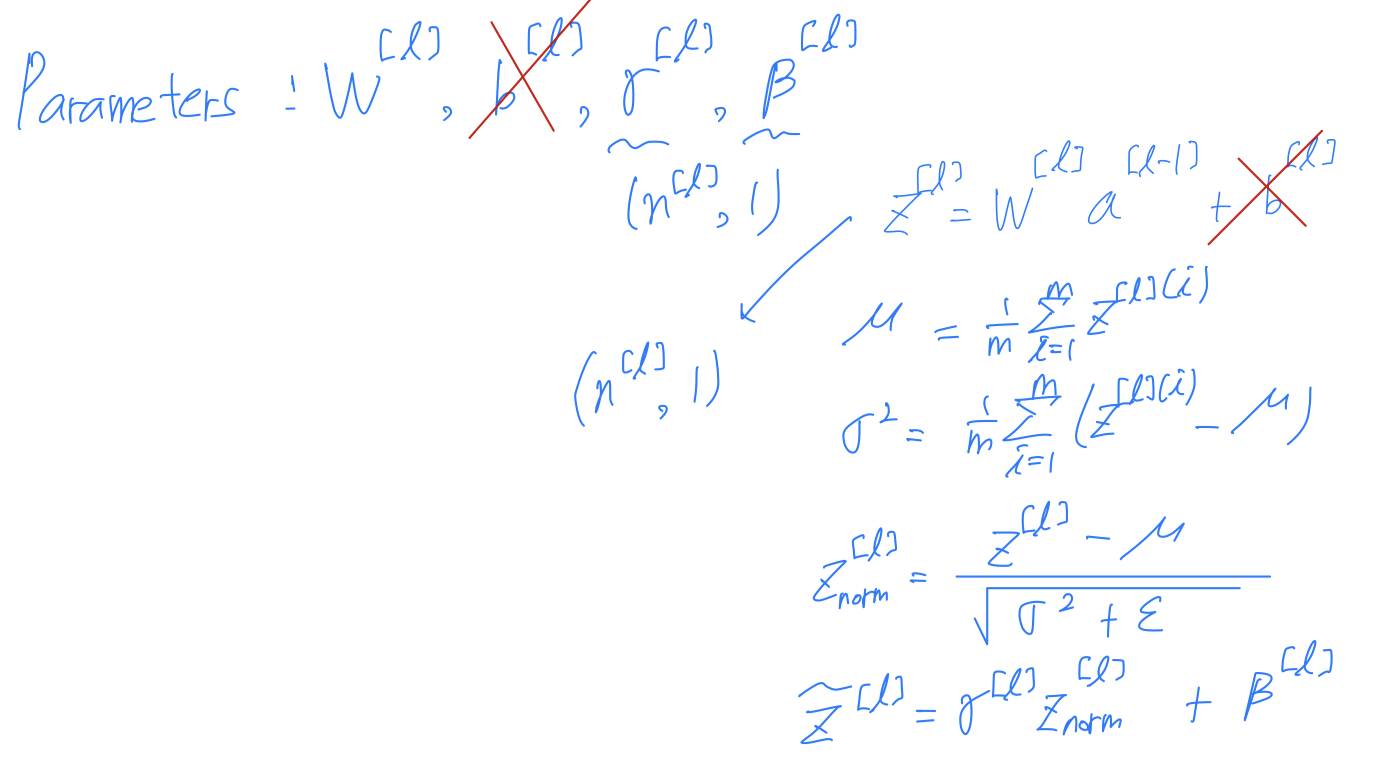

Implementing gradient descent

• So, let's put all together and describe
  how you can implement gradient descent using Batch Norm.
  

---

Why does Batch Norm work?

• So why does batch norm work?
  Here's one reason,
  you've seen how normalizing the input features,
  the $X$, to mean $0$ and variance $1$, how that can speed up learning.
  So rather than having some features that range from $0$ to $1$,
  and some from $1$ to $1,000$, by normalizing all the features.
  Input features $X$ to take on similar range of values that can speed up learning.
  ($X$가 비슷한 범위의 값을 갖고, 학습 속도가 증가)
  So one intuition behind why batch norm works is,
  this is doing a similar thing, but further values in hidden units and not just for your input layer.
  This is just a partial picture for what batch norm is doing.
  There are couple of further intuitions, that will help you gain a deeper understanding of what batch norm is doing.

• A second reason why batch norm works is it makes weights later or deeper thatn your networks,
  Let's see a training on network, a shalllow network like logistic regression or a neural nework.
  Let's say that you've trained your data sets on all images of black cats.
  (검은 고양이 사진만으로 훈련했다고 가정.)
  If you now try to apply this network to data with colored cats,then your cost might not do very well.
  (만약 색깔있는 고양이를 test한다면, cost가 잘 동작하지 않을 수 있다.)
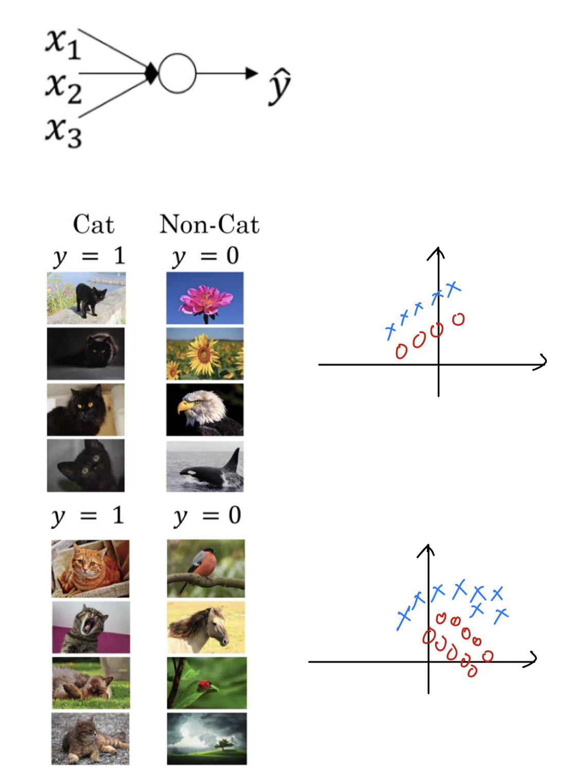  You might not expect a module trained on the data on the black to do very well on the data on the colored.
  So this idea of your data distribution changing goes by the somewhat fancy name,
  convariate shift.
  (데이터의 분포가 변하는 아이디어를 covariate shift라고 한다.)
  And the idea is that, if you learned some $X$ to $Y$ mapping,
  if the distribution of $X$ changes, then you might need to retain your learning algorithm.
  (만약 X에서 Y로 가는 매핑을 배운 경우에 X의 분포가 변경되면 학습 알고리즘을 다시 훈련시켜야 한다.)
  And this is true even if the function, the ground truth function, mapping from $X$ to $Y$,
  remains unchanged, which it is in this example.
  (위의 고양이 예제와 같이 ground truth 함수가 변하지 않더라도 X의 분포가 바뀌면, 다시 훈련시켜야 한다.
  ground truth 함수는 그림이 고양이인지 아닌지에 대한 것이기 때문에)
  And the need to retain your function becomes even more acute(격렬한, 심한) or
  it becomes even worse if the ground truth function shifts as well.
  (ground truth 함수도 함께 shift되면 더욱 함수를 다시 유지시켜야할 필요성이 강해진다.)
  
  So how does this problem of covariate shift apply to a neural network?

Why this is a problem with neural networks?

• Let's look at the learning process from the perspective of the third hidden layer.
  So this network has learned the parameters $W^{[3]}$ and $b^{[3]}$
  And from the perspective of the third hidden layer,
  it gets some set of values from the earlier layers,
  and then it has to do some stuff to hopefully make the output $\hat{Y}$ close to ground truth value $Y$.
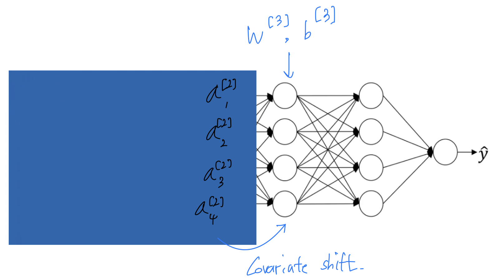  이전 node들을 잠시 가려보자.
  So from the perspective of this third hidden layer, it gets some values,
  let's call them $a^{[2]}_1, a^{[2]}_2, a^{[2]}_3, a^{[2]}_4$.
  But these values might well be features $x_1, x_2, x_3, x_4$, and the job of the third hidden layer
  is to take these values and find a way to map them to $\hat{Y}$.
  The network is also adpating parameters $W^{[2]}, b^{[2]}$ and $W^{[1]}, b^{[1]}$,
  and so as these parameters change, these values $A^{[2]}$ will also change.
  So from the perspective of the third hidden layer,
  these hidden unit values are changing all the time,
  and so it's suffering from the problem of covariate shift.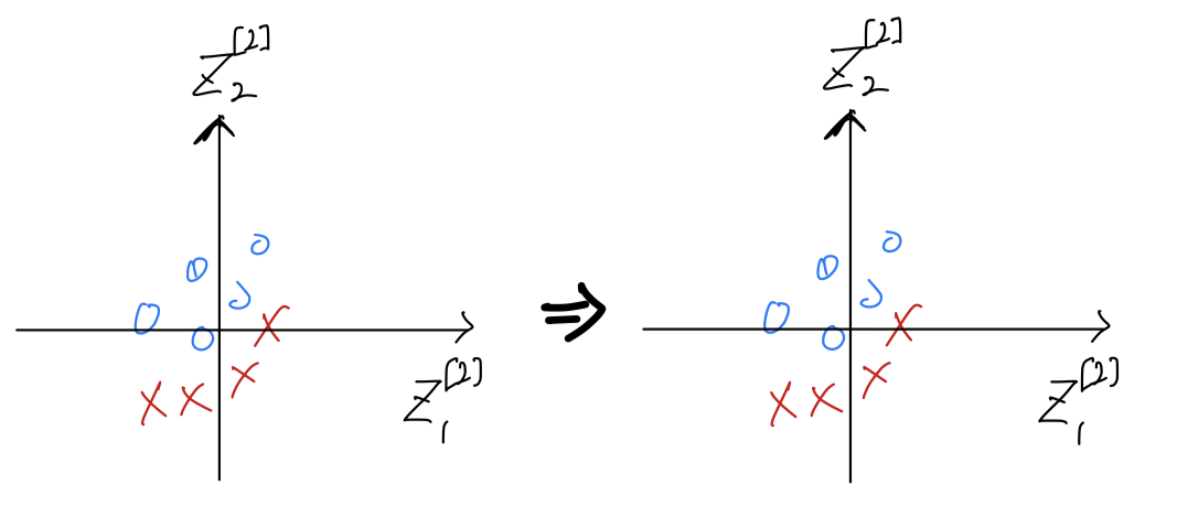($Z^{[2]}$는 4개의 원소가 있는데, 간략화하여 2개로 시각화)
  So what batch norm does is
  it reduces the amount that the distribution of these hidden unit values shifts around.
  And if it were to plot the distribution of these hidden unit values,
  maybe this is technically renormalizer $Z$.
  The values for $z^{[2]}_1, z^{[2]}_2, z^{[2]}_3, z^{[2]}_4$ can change,
  and indeed they will change when the neural network updatees the parameters in the earlier layers.
  But what batch norm ensures is that no matter how it changes,
  the mean and variance of $z^{[2]}_1, z^{[2]}_2, z^{[2]}_3, z^{[2]}_4$ will remain the same.
  (신경망이 update하면서 이전 layer들의 값들도 변할 것인데,
  Batch Norm은 그것들이 어떻게 변하더라도 $Z^{[2]}$의 mean과 variance를 똑같을 거라는 것을 보장해준다.
  즉, $Z^{[2]}$의 값이 변하더라도 $Z^{[2]}$는 $\gamma^{[2]}$, $\beta^{[2]}$에 의해 정해진 mean과 variance의 값을 계속 유지할 것이다.)
  What this does is,
  it limits the amount to which updating the parameters in the earlier layers can affect the distribution of values that the third layer now sees and has to learn on.
  (이전의 layer에서 parameter가 update되면서 세번째 layer에 영향을 줄 수 있는 양을 제한시켜 준다.
  그 양은 세번째 layer가 새로 배워야 하는 양이기도 하다.)
  And so, batch norm reduces the problem of the input values changing,
  it really causes these values to become more stable,
  so that the later layers of the neural network has more firm ground to stand on.
  (deeper layer들이 그 자리를 지킬 수 있는 틀을 마련해준다.)
  And even though the input distribution changes a bit, it changes less,
  and what this does is, even as the earlier layers keep learning.
  (그리고 비록 입력값의 분포도가 약간 변하기는 하지만, 더 작게 변하고,
  이것이 하는 일은 이전 층의 parameter들이 계속 변하는데, 그로 인해 다음 층들이 update해야 하는 양이 줄어들게 된다.)
  It weakens the coupling between what the early layers parameters have to do and
  what the later layers parameters have to do.
  And so it allows each layer of the network to learn by itself, a little bit more independently of other layers,
  and this has the effect of speeding up of learning in the whole network.
  (earlier layer에서 수행해야 하는 작업과 later layer에서 수행해야 하는 작업을 줄여준다.
  따라서 network의 각 layer들이 조금 더 독립적으로 스스로 학습할 수 있게 된다.
  결과적으로 전체 network의 속도를 올려주는 효과를 준다.)
  The earlier layers don't get to shift around as much,
  because they're constrained to have the same mean and variance.
  And so batch norm makes the job of learning on later layers easier.
  (earlier layer는 똑같은 평균과 분산을 갖도록 제한되어 있기 때문에 covariate shift 폭이 크지 않기 때문에
  batch norm의 진정한 의의는 later layer의 학습을 쉽게 해준다는 것이다.)
  
  

Batch Norm as regularization

• It turns out batch norm has a second effect.
  It has a slight regularization effect.
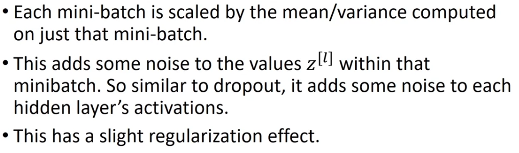  mini-batch $X^{\{t\}}$는 $Z^{\{t\}}$를 갖게 되는데,
  해당 mini-batch만의 mean과 variance이 계산되기 때문에 그 mean과 variance에는 약간의 noise가 있다.
  마찬가지로 $Z^{\{t\}[l]}$에 약간의 noise가 있기 때문에,
  noiser가 있는 mean과 variance를 사용하여 계산된 $\tilde{Z}^{{\{t\}[l]}}$에도 noise가 있다.
  그래서 Dropout과 비슷하게 each hidden layer's activations에 some noise를 추가하여 slight generalization 효과가 있다.
  Because by adding noise to the hidden units,
  it's forcing the downstream hidden units not to rely too much on any one hidden unit.
  And so simliar to dropout, it adds noise to the hidden layers and therefore has a very slight regularization effect.
  Because the nois added is quite small, this is not a huge regularization effect,
  and you might choose to use batch norm together with dropout if you want the more powerful regularization effect of dropout.
  
  So if you use a mini-batch size of 512 instead of 64, by using a larger mini-batch size,
  you're reducing this noise and therefore also reducing this regularization effect.
  (더 큰 mini-batch size를 쓰게 되면 noise가 줄게 되고 regularization effect도 줄어든다.)
  So that's one strange properety of dropout which is that by using a bigger mini-batch size,
  you reduce the regularization effect.
  (그래서 mini-batch size를 크게하면 regularization 효과가 줄어들게이 dropout의 이상한 속성 중 하나이다.)
  
  Really, don't use to batch norm as a regularization.
  Use it as a way to normalize your hidden units activations and therefore speed up learning.
  (Batch Norm은 약간의 regularization 효과가 있지만, regularizor로 사용하지는 않을 것이다.
  Batch Norm을 사용하는 진짜 의도는 regularization이 아니기 때문이다.
  따라서 Batch Norm은 학습 속도를 높이기 위한 hidden units의 normalization하는 수단으로 사용하라.)

---

Batch Norm at test time

• Batch Norm은 한 번에 하나의 mini-batch로 처리하지만,
  test time에는 한 번에 하나의 example에 대해서 처리해야 할 수도 있다.
  Let's see how you can adapt your network to do that.

• Here are the equations you'd use to implement batch norm.
  Notice that $\mu$ and $\sigma^2$ which you need for this scaling caculation
  are computed on the entire mini-batch.
  But the test time you might not have a mini-batch of 64, 128 or 256 examples to process at the same time.
  So, you need some different way of coming up with $\mu$ and $\sigma^2$.
  And if you have just one example, taking the mean and variance of that one example doesn't make sense. (1개의 값을 가지고 계산하는 것은 말이 안된다.)
  
  In order to apply your neural network and test time is to come up with some separate estimate of $\mu$ and $\sigma^2$,
  so what's actually done?
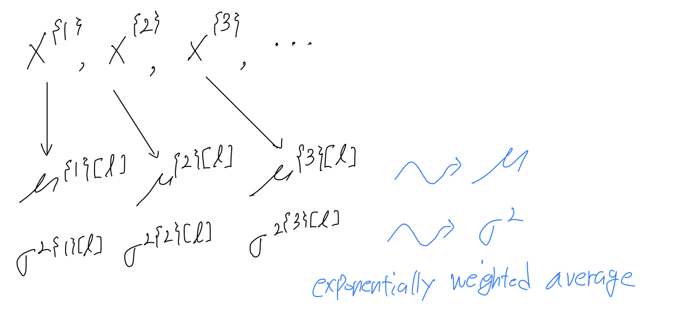  ➡️ what you do is estimate this using a exponentially weighted average
  where the average is across the mini-batches.
  Let's pick some layer $L$ and let's say ou're going through mini-batches $X^{\{1\}}$.
  So that exponentially weighted average becomes your estimate for what the mean of the $Z$ is for that hidden layer
  and similarly, you use an exponentially weighted average to keep trakc of variance.
  So you keep a running average of the $\mu$ and $\sigma^2$ that you're seeing for each layer as you train the neural network across different mini-batches.
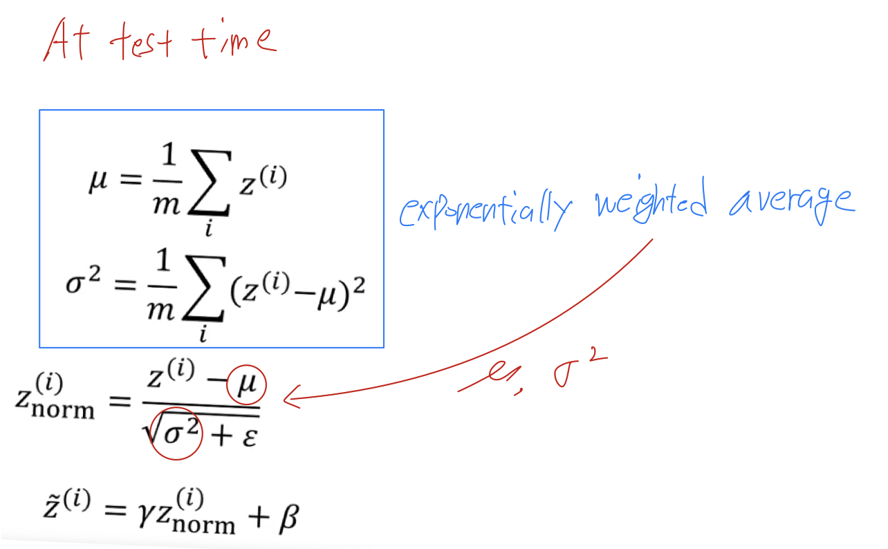  Then finally at test time, what you do is in place of this equation,
  you would just compute $z_{norm}^{{\{t\}[l]}(i)}$ using your exponentially weighted average of the $\mu$ and $\sigma^2$.
  So the takeaway from this is that
  during training time $\mu$ and $\sigma^2$ are computed on an entire mini-batch of say 64, 128 or some number of examples.
  But the test time, you might need to process a single example at a time.
  So, the way to do that is to estimate $\mu$ and $\sigma^2$ from your training set and there are many ways to do that.
  In practice, what people usually do is implement and exponentially weighted average where you just keep track of $\mu$ and $\sigma^2$ during training,
  also sometimes called the running average.
  In practice, this process is pretty robust to the exact way you used to estimate $mu$ and $\sigma^2$.
  So i wouldn't worry too much about exactly how you do this and if you're using a deep learning framework,
  they'll usually have some deafult way to estimate the $\mu$ and $\sigma^2$ that should work reasonably well as well.

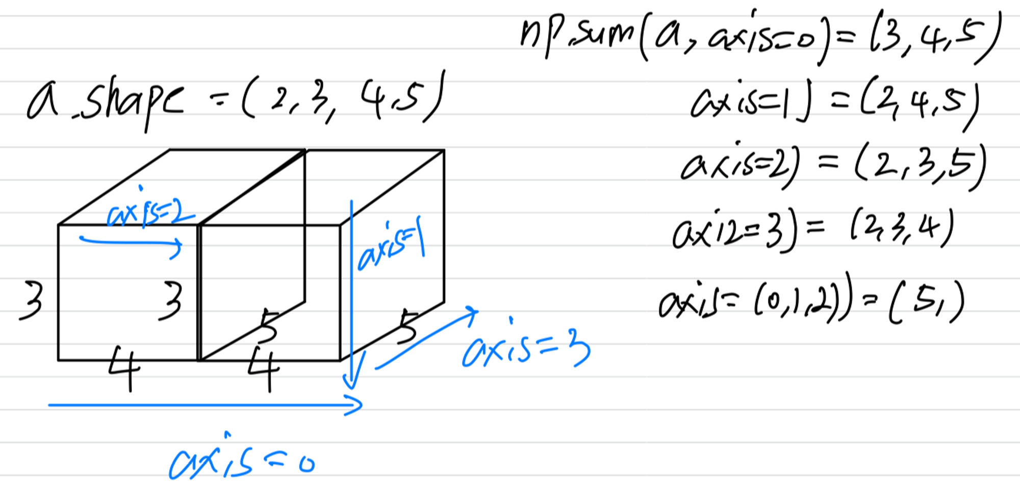
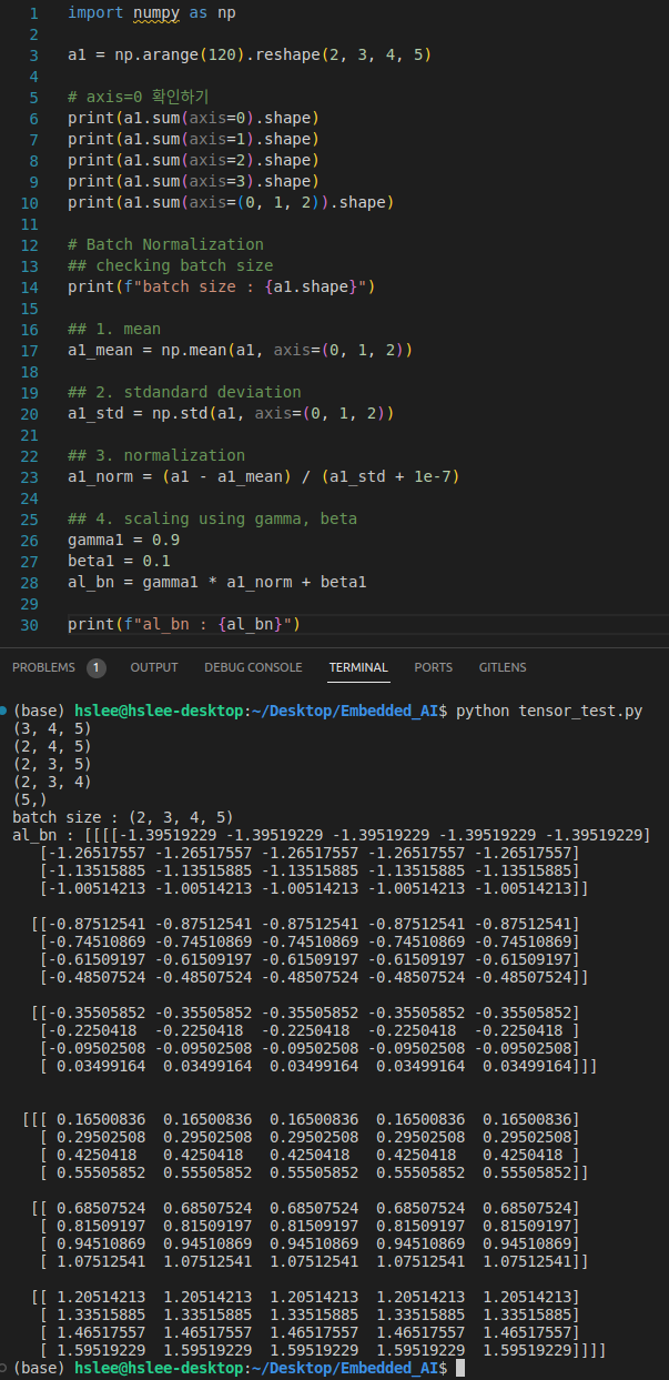
Numpy Experiment

•