Week 2 | Optimization Algorithms

HyungSeop Lee·2023년 7월 28일

Problem of Plateaus RMSProp adam bias correction exponentially weighted average learning rate decay momentum

[Coursera | DL Specialization | 2 ] Improving Deep Neural Networks: Hyperparameter Tuning, Regularization and Optimization

목록 보기

3/8

Mini-batch Gradient Descent

You've learned previously that vectorization allows you to efficiently compute on all $m$ examples,
that allows you to process your whole training set without an explicit For loop.
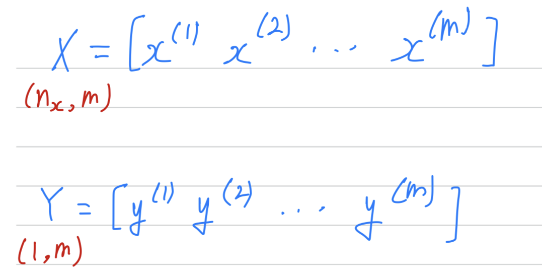
So that's why we would take our training examples and stack them
into these huge matrix $X, Y$
Vectorization makes you to process all $m$ examples quickly if $m$ is large then it can still be slow.
For example what if $m$ was 5,000,000 or even bigger.
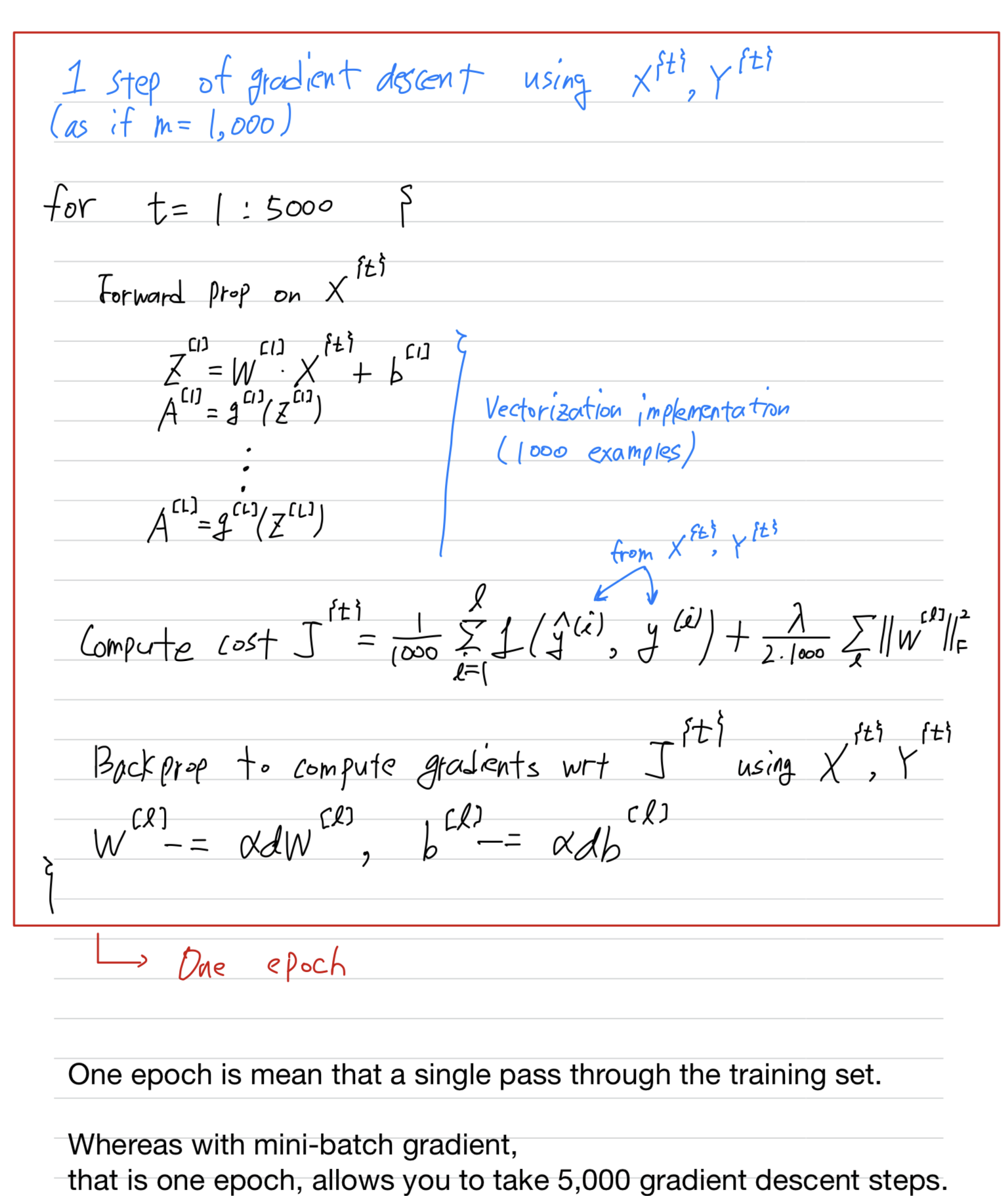
With the implementatino of gradient descent on your whole trainin set,
what you have to do is you have to process your entire training set
before you take one little step of gradient descent.
And then you have to process your entire training sets of 5,000,000 samples again before you take another little step of gradient descent.

So, it turns out that you can get a fastser algorithm if you let gradient descent start to make some progress even before you finish processing your entire, your giant graining sets of 5,000,000 examples.

In particular, here's what you can do.
Let's say that you split up your training set into smaller,
and theses baby training sets are called mini-batches.
And let's say each of your baby training sets have just 1,000 examples each.
So, you take $x_1$ through $x_{1,000}$ , and you call that your first mini-batch,
And then you take next $x_{1,001}$ through $x_{2,000}$ and come next one and so on.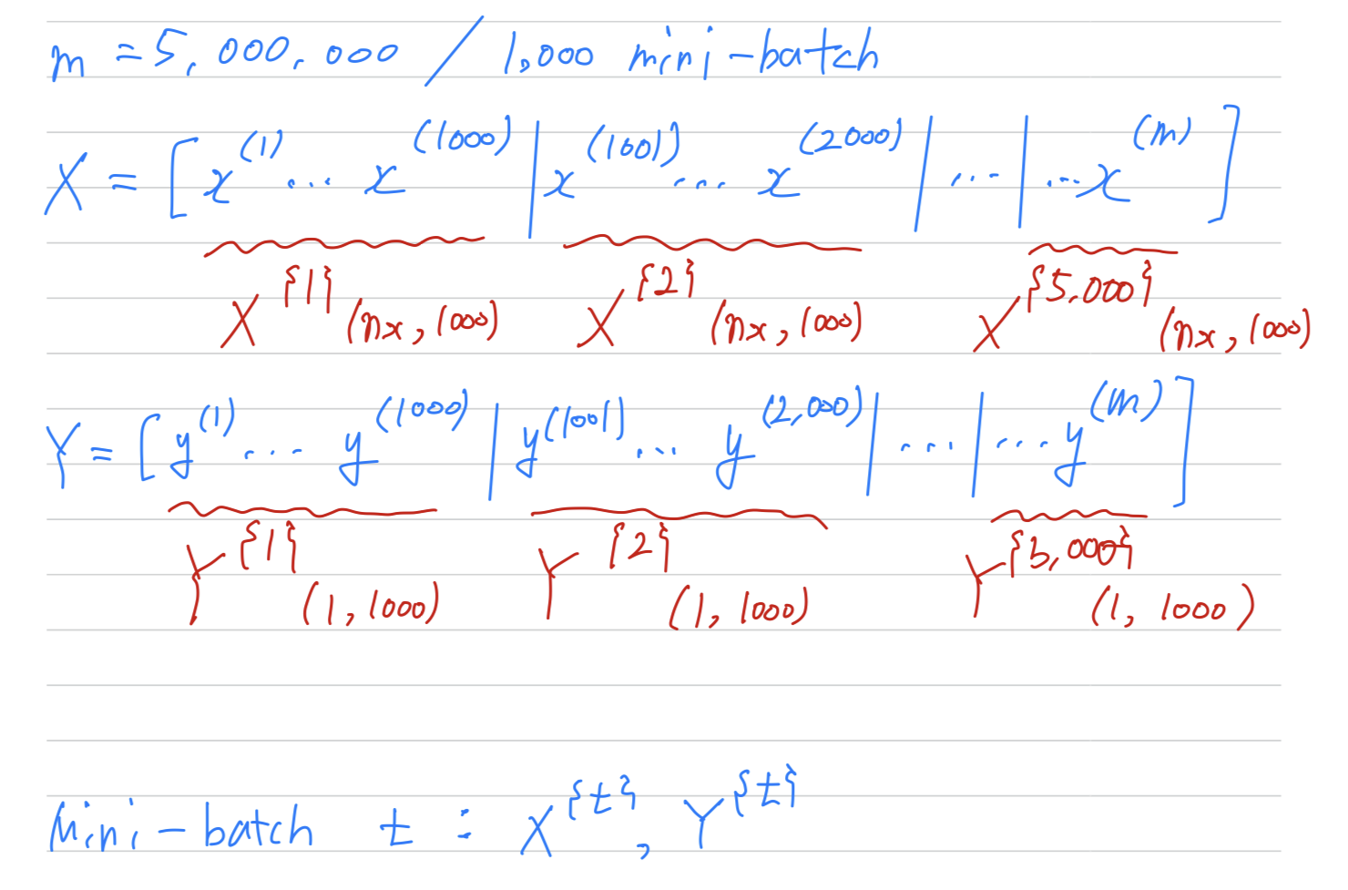To explain the name of this algorithm,
Batch gradient descent, refers to the gradient descent algorithm
we have been talking about previously
where you process your entire training set all at the same time.
And the name comes from viewing that as processing your entire batch of training samples all at the same time.
Mini-batch gradient descent in contrast, refers to algorithm
which you process single mini-batch $X^{\{ t \}}, Y^{\{ t \}}$ at the same time
rather than processing your entire training set $X, Y$ the same time.

So, let's see how mini-batch gradient descent works.

Understanding Mini-batch Gradient Descent

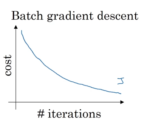
With batch gradient descent on every iteration you go through the entire training set and you'd expect the cost to go down on every ingle iteration.
So if we've had the cost funtion $J$ as a function of different iterations
it should decrease on every single iteration.
And if it ever goes up even on iteration then something is wrong.
On mini-batch gradient descent though,
if you plot progress on your cost function,
then iy may not decrease on every iteration.
In particular, on every iteration you're processing some $X^{\{t\}}, Y^{\{t\}}$
and so if you plot the cost function $J^{\{t\}}$ which is computer using just $X^{\{t\}}, Y^{\{t\}}$ .
So you plot the cost function $J$ , you're more likely to see something that looks like this.
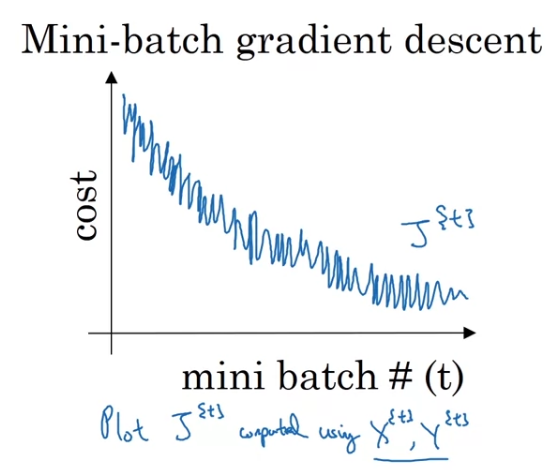It should trend downwards, but it's also going to be a little bit noisier.
So if you plot $J^{\{t\}}$ ,
as you're training mini-batch gradient descent may be over multiple epochs,
you might expect to see a curve like this.
So it's okay if it doesn't go down on every iteration.
The reason it'll be a little bit noisy is that,
maybe $X^{\{1\}}, Y^{\{1\}}$ is just the rows of easy mini-batch
so your cost might be a bit lower.
But then maybe just by chance, $X^{\{2\}}, Y^{\{2\}}$ is jjust a harder mini-batch.
Maybe you needed some mislabeled examples in it, in which case the cost will be a bit higher and so on.
( $X^{\{1\}}, Y^{\{1\}}$ 보다 $X^{\{2\}}, Y^{\{2\}}$ 에 잘못된 레이블이 더 많을 수도 있기 때문 ➡️ noisy, oscillation)
So that's why you get these oscillations as you plot the cost when you're running mini-batch gradient descent.

Choosing your mini-batch size

Now one of the prarmeters you need to choose is the size of your mini-batch.

Two extremes

If the mini-batch size = $m$ , then you just end up with batch gradient descent.
So in this extreme you would just have one mini-batch $X^{\{1\}}, Y^{\{1\}}$
and this mini-batch is equal to your entire training set.
So setting a mini-btach size $m$ just gives you batch gradient dsecent.
- So let's look at what these two extremes will do on optimizing this cost function.
  If these are the contours of the cost function you'r trying to minimize.
  Then batch grdient descent might start somewhere
  and be able to take relatively low noise, relatively large steps.
- If you use batch gradient descent(mini-batch size = $m$ ),
  then you're processing a huge training set on every iteration.
  So the main disadvantage of this is that it takes too much time too long per iteration
  assuming you have a very long training set.
  If you have a small training set, then batch gradient descent is fine.
If your mini-batch size = $1$ , this gives you an algorithm called stochastic gradient descent.
And here every example is its own mini-batch.
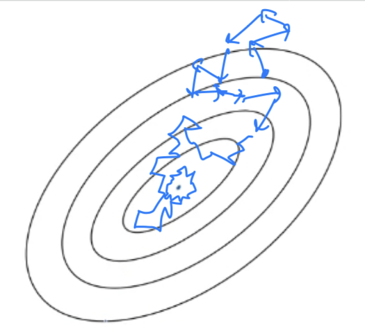
So whay you do in this case is you look at first mini-batch, $(X^{\{1\}}, Y^{\{1\}})$ = $(x^{(1)}, y^{(1)})$
- In contrast with stochastic gradient descent
  then on every iteration you're taking gradient descent with just a single training example so most of the time you hit two of the global minimum.
  But sometime you hit in the wrong direction if that one example happens to point you in a bad direction.
  So stochastic gradient descent can be extremely noisy.
  And on average, it'll take you in a good direction,
  but sometimes it'll head in the wrong direction as well.
  As stochastic gradient descent won't ever converge(수렴하지 않는다),
  it'll always just kind of oscillate and wander around the region of the minimum.
  But it won't ever just head to the minimum and stay there.
- If you use stochastic gradient descent(mini-batch size = $1$ ),
  then it's nice that you get to make progress after processing just one example.
  That's actually not a problem.
  And the noisiness can be ameliorated(개선되돠) or can be reduced
  by just using a smaller learning rate.
  But a huge disadvantage to stochastic gradient descent is that
  you lose almost all your speed up from vectorization.
  Because, here you're processing a single training example at a time.
  The way you process each example is going to be very inefficient.

So what works best in practice is something in between where you have some,
Mini-batch size not too big or too small.
And this gives you in practice the fastest learning.
And you notice that this has two good things going for it.
1. One is that you do get a lot of vectorization.
  So in the example we used on the previous video,
  if your mini-batch size = $1,000$ examples then,
  you might be able to vectorize across $1,000$ examples
  which is going to be much faster than processing the examples one at a time.
2. And second, you can also make progress
  without needing to wait until you process the entire training set.
  So again using the numbers we have from the previous video,
  each epoch or each parts your training set allows you
  to see $5,000$ gradient descent steps.
So in practice they'll be some in-between mini-batch size that works best.
(따라서 실제로 가장 잘 작동하는 적당한 mini-batch size가 있을 것이다.)
It's not guaranteed to always head toward the minimum
but it tends to head more consistently in direction of the minimum
than the consequent descent.
And then it doesn't always exactly converge or oscillate in a very small region.
If that's an issue you can always reduce the learning rate slowly.
(We'll talk more about how to reduce the learning rate in later video.)

Choosing your mini-batch size

So if the mini-batch size should not be $m$ and should not be $1$
but should be something in-between,
how do you go about choosing it?
Here are some guidlines.

First, if you have a small training set( $m \lt 2,000$ ),
Just use batch gradient descent.
If you have small training set then
no point using mini-batch gradient descent you can process a whole training set quite fast.
So you migh as well use batch gradient descent.
Otherwise, if you have a bigger training set,
typical mini-batch sizes would be $(64=2^6, 128=2^7, 256=2^8, 512=2^9)$ are quite typical.
And because of the way computer memory is layed out and accessed,
sometimes you code runs faster if your mini-batch size is a power of $2$ .
So often i'll implement my mini-batch size to be a power of $2$ .
In a previous video we used a mini-batch size of $10,000$ ,
if you really wanted to do that i would recommend you just use your $1,024(2^{10})$
One last tips is to make sure that your mini-batch( $X^{\{t\}}, Y^{\{t\}}$ ) fits in CPU/GPU memory.
And this really depends on your application and how large a single training sample is.
But if you ever process a mini-batch that doesn't actually fit in CPU, GPU memory,
whether you're using the process, the data.
Then you find that the performance wuddenly falls of a cliff and is suddenly much worse.

Exponentially weighted averages

I want to show you a few optimization algorithms.
They are faster than gradient dsecent.
In order to understand those algorithms, you need to be able they use something called exponentially weighted averages
(= exponentially weighted moving averages in statistics).
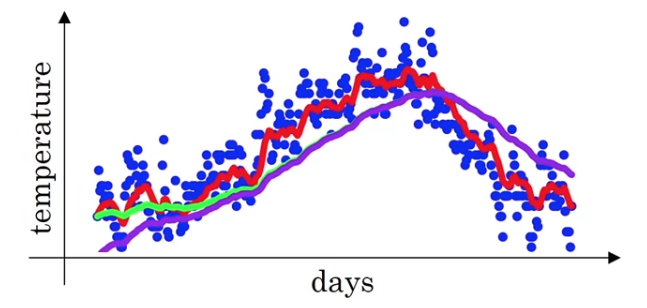
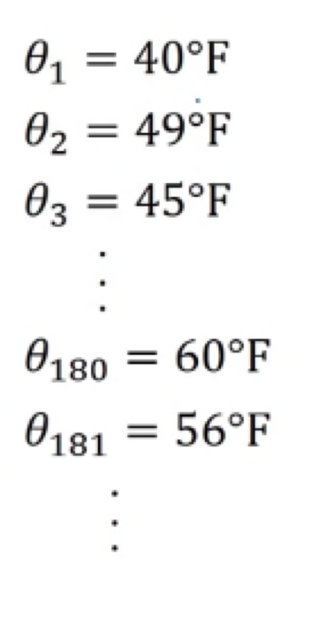
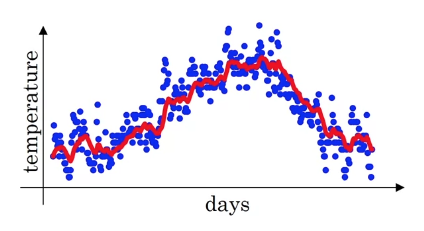
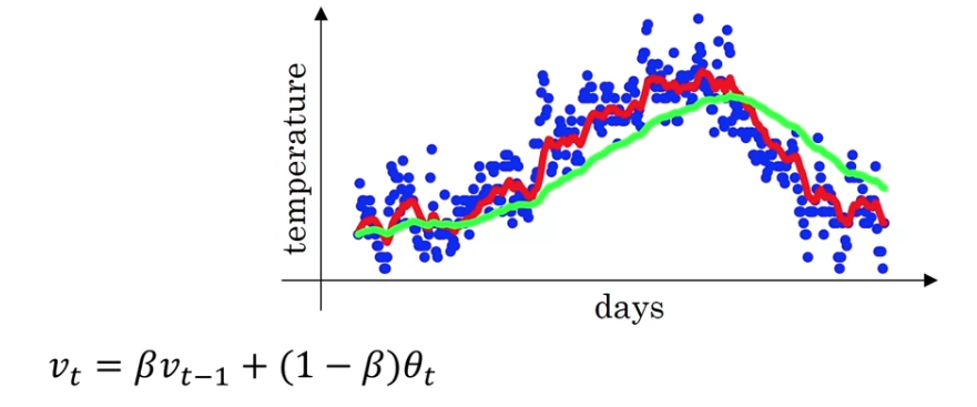
For this example i got the daily temperature from London from last year.
So, on January 1, temperature was 40 degree Fahrenheit(화씨).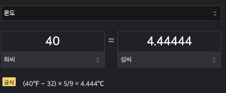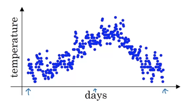So you plot the data you end up with this.
This data looks a little bit noisy and if you want to compute the trends,
the local average or a moving average of the temperature,
here's what you can do.
Let's initialize $V_0=0$ .
And then, on every day, $V_1 = 0.9V_0 + 0.1\theta_{temperaturefromtheday}$
On the firsy day, $V_1 = 0.9V_0 + 0.1\theta_{1}$
And on the second day, $V_2 = 0.9V_1 + 0.1\theta_{2}$
And on the third day, $V_3 = 0.9V_2 + 0.1\theta_{3}$ , ...
And the more general formula is
$V_{t} = 0.9V_{t-1} + 0.1\theta_{t}$

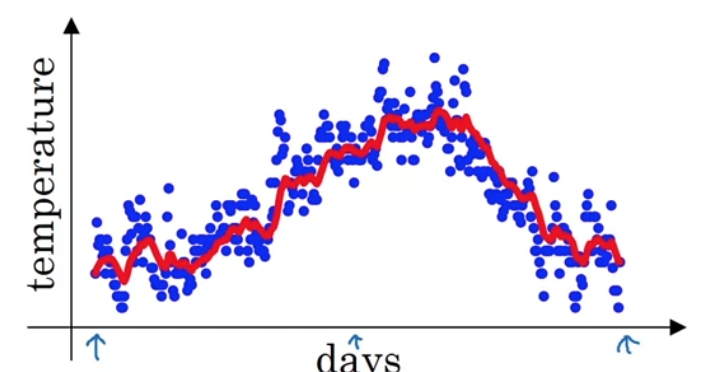
So if you compute this and plot it red, this is what you get.
You get a moving average of what's called an exponentially weighted average of the daily temperature.
So let's took at the equation we had from the previous slide,
$V_t = \beta V_{t-1} + (1-\beta)\theta_t$
$\beta=0.9$
It turns out that for reasons we going to later,
when you compute this you can think of $V_t \simeq \frac{1}{1-\beta}days temperature$
- So, for example when $\beta=0.9$ ,
  you could think of this as averaging over the last 10days temperature.
  And that was the red line.
- Let's set $\beta$ to be very close to $1$ , let's say $\beta = 0.98$ .
  Then, if you look at $\frac{1}{1-0.98}=50$
  So, this is think of this as averaging over roughly, the last 50 days temperature.
  And if you plot that you get this green line.
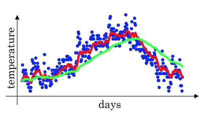  So notice a couple of things with this very high value of $\beta$ .
  1. The plot you get is much smoother
  because you're now averaging over more days of temperature.
  2. but on the flip side the curve has now shifted further to the right.
  because you're now averaging over a much larger window of temperatures.
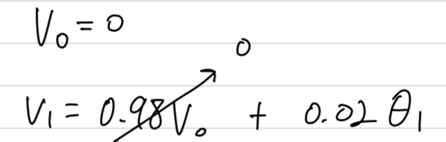
  And the reason for that is when $\beta=0.98$
  then it's giving a lot of weight to the previous value and a much smaller weight just 0.02 to whatever you're seeing right now.
  So when the temperature changes,
  ther's exponentially weighted average just adapts more slowly when $\beta$ is so large.
  So, there's just a bit more latency.
- Now, let's say $\beta=0.5$ ,
  then, if you look at $\frac{1}{1-0.5}=2$
  So, this is something like averaging over just $2$ days temperature,
  and you plot that you get this yellow line.
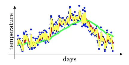  And by averaging only over two days temperature,
  you have a much, as if you're averaing over much shorter window.
  So, you're much more noisy, much more susceptible(허락한다) to outliers.
  But this adapts much more quickly to what the temperature changes.
  So, this formula is highly implemented, exponentially weighted average.
By varing this hyperparameter( $\beta$ )
you can get slightly different effects and there will usually be some value in between that works best.

Understanding exponentially weighted averages

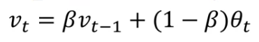
Recall that this is a key equation for implementing exponentially weighted averages.

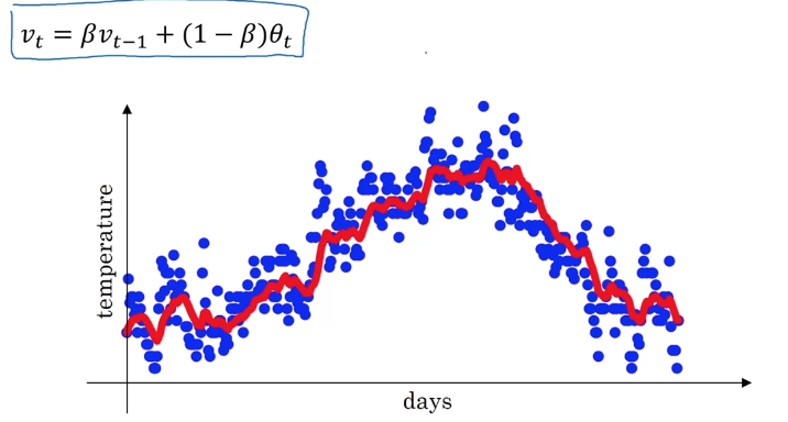
This will turn out be a key component of several optimization algorithms
that you used to train your neural networks.
So, i want to develop a little bit deeper into intuitions for what this algorithm is really doing.
Here's an equation again and let's set $\beta=0.9$ and write out a few equations that this corresponds to.
To analyze it, i've written it with decreasing values of $t$ .
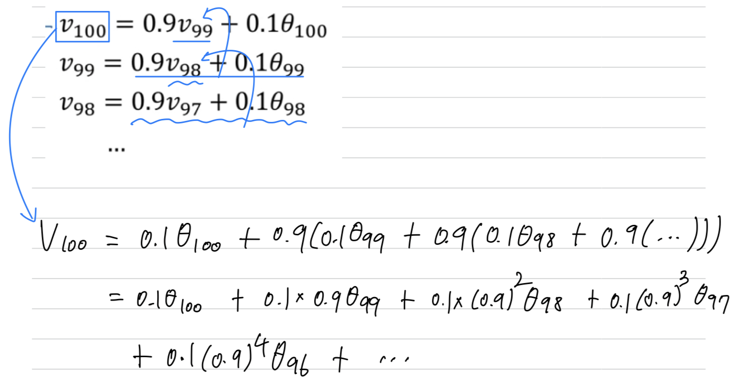
Because of that, this really is an exponentially weighted average.
And finally, you might wonder, how many days temperature is this averaging over.
It turns out that $0.9^{10} \simeq 0.35 \simeq \frac{1}{e}$
And, more generally,
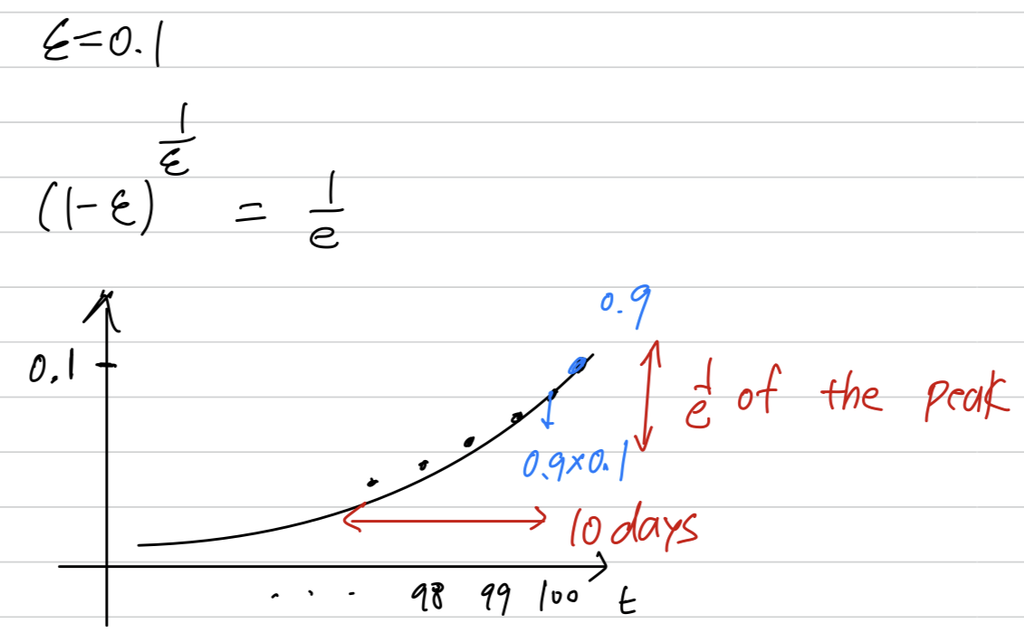it takes about 10 days for the height of this to decay to $\frac{1}{e}$ of the peak.

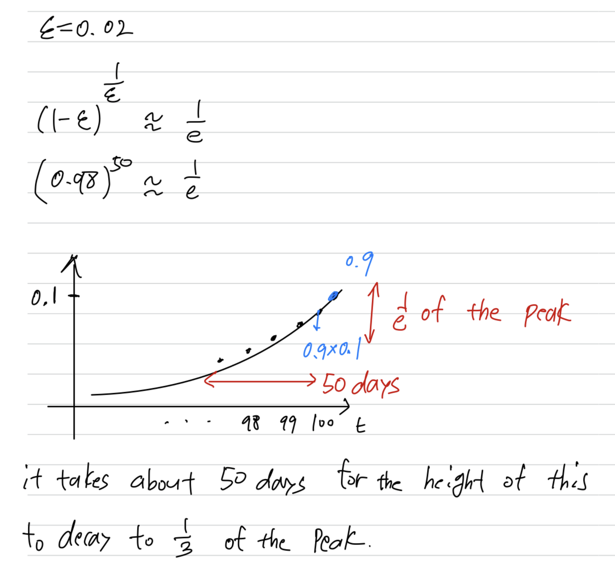Whereas, in contrast, if $\beta = 0.98$ ,
then, what do you need $0.98^{?}$ in order for this to really small?
Turns out $0.98^{50} \simeq \frac{1}{e}$ .
So the way to be pretty bigwill be bigger than $\frac{1}{e}$ for the first 50 days,
and then they'll decay quite rapidly over that.
because, in this example, to use the notation $(1-\epsilon)^{\frac{1}{\epsilon}}$
it's as if $\epsilon=0.02$

And this, by the way, is how we got the formula
that we're averaging over $\frac{1}{1-\beta}$ or so days.
$\epsilon$ replace a row of $\epsilon = 1-\beta$
It tells you,
up to some constant roughly how many days temperature you should think of this as averaging over.
(대략적으로 며칠 동안의 온도를 평균으로 생각해야 하는지를 알려준다)
But this is just a rule of thumb for how to think about it,
and it isn't a formal mathematical statement.

Implementing exponentially weighted averages

Finally, let's talk about how you actually implement this.
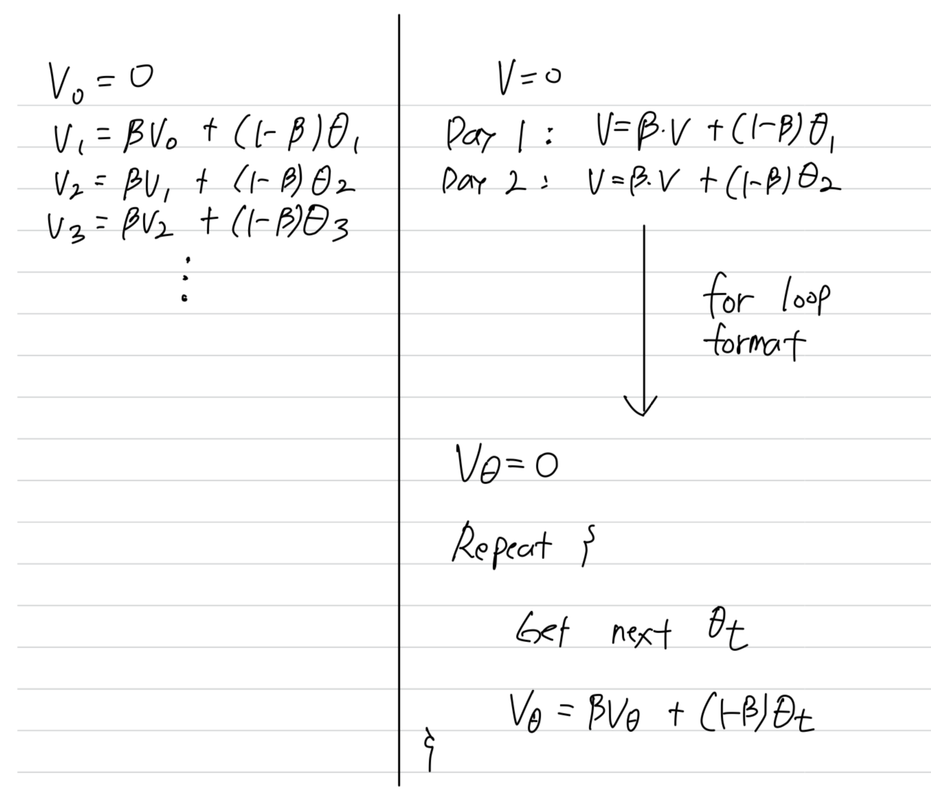So one of the advantages of this exponentially weighted average formula is
that it takes very little memory.
You just need to keep just one real number( $V_{\theta}$ ) in computer memory,
and you keep on overwriting it with this formula( $V_{\theta}=\beta V_{\theta} + (1-\beta)\theta_{t}$ )
based on the latest values that you got.
It's really not the best way, not the most accurate way to compute an average.
If you were to compute a moving window,
where you explicitly sum over the last 10 days, the last 50 days temperature
and just divide by 10 or 50,
that usually gives you a better estimate.
But the disadvantae of that,
of explicitly keeping all the temperatures around and sum of the last 10 days is it requires more memory,
and it's just more complicated to implement and is computationally more expensive.

So for things, we'll see examples on the next few videos,
where you need to compute averages of a lot of variables.
This is a very efficient way to do so both
from computation and memory efficiency point of view which is it's used in a lot of machine learning.

Bias correction in exponentially weighted average

You've had learned how to implement exponentially weighted average.
There's one technical detail called bias correction that
can make your computation of these averages more accurately.
In the previous video, you saw this figure for
$\beta=0.9$
$\beta=0.98$
But it turns out that if you implement the formula as written here,
you won't actually get the green curve when $\beta=0.98$
you actually get the purple curve here.
You notice that the purple curve starts off really low.
So let's see how to fix that.
When implementing a moving average,
That's why if the first day's temperature is 40 degrees Fahrenheit,
then $V_1 = 0.02 * 40$ which is $0.8$ , so you get a much lower value down here.
That's not a very good estimate of the first day's temperature.![]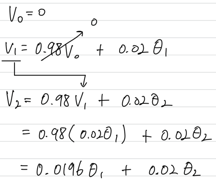Assuming $\theta_1, \theta_2 > 0$
When you compute $V_2$ , it will be much less than $\theta_1$ or $\theta_2$
so $V_2$ isn't a very good estimate of the first two days temperature of the year.
It turns out that there's a way to modify this estimate that makes it much better(accurate),
especially during this initial phase of your estimate.

Instead of taking $V_t$ , take $\frac{V_t}{1-\beta^t}$ (where $t$ is the current day that you're on.)
Let's take a concrete example.
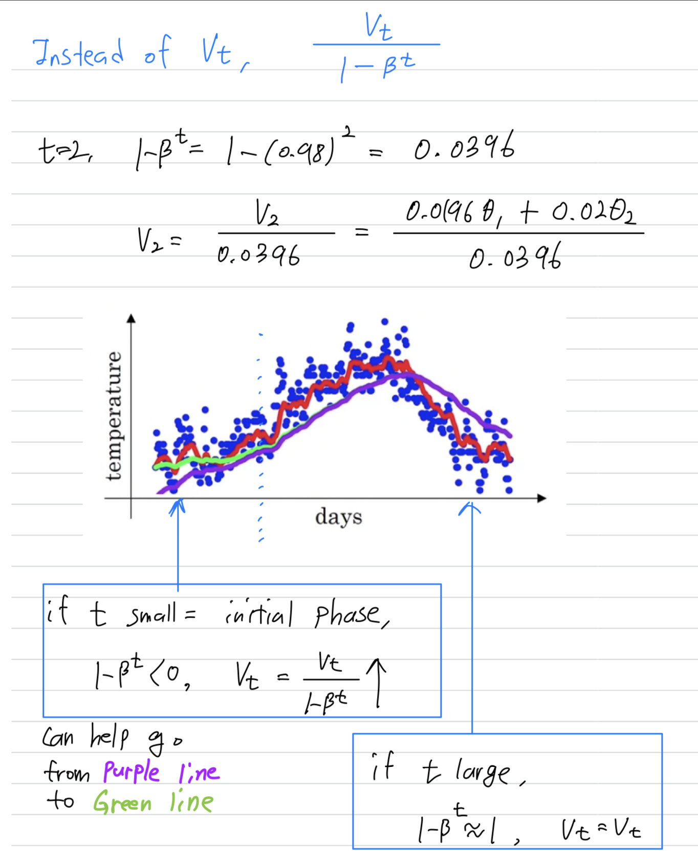You notice that as $t$ becomes large, $\beta^t \simeq 0$ , the bias correction makes almost no difference.
This is why when $t$ is large, the purple line and the green line pretty much overlap.
But during this initial phase of learning,
bias correction can help you obtain a better estimate of the temperature.
This is bias correction can help you go from the purple line to the green line.

Gradient descent with momentum

There's an algorithm called momentum, or gradient descent with momentum
that almost always works faster than the standard gradient descent algorithm.
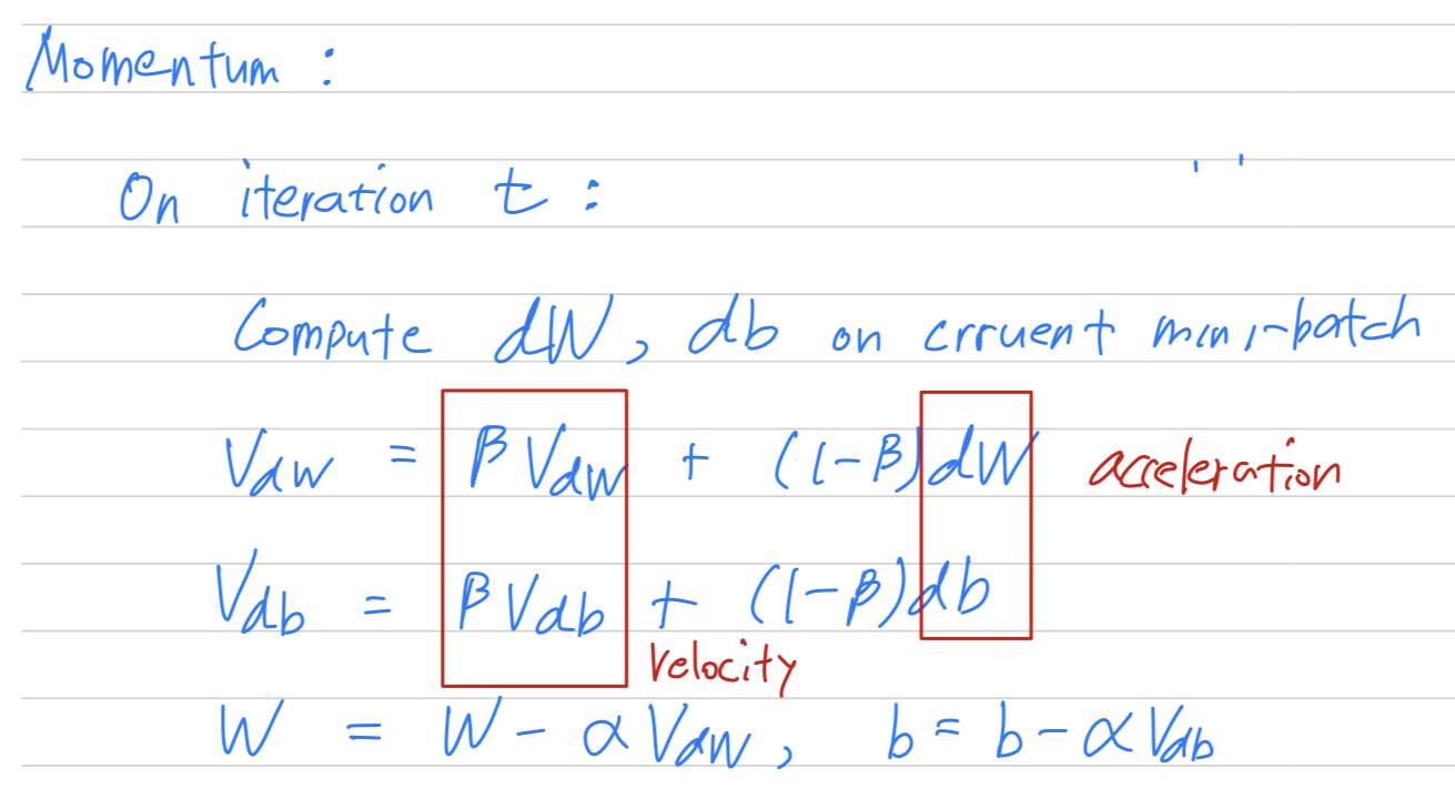
The basic idea is to compute an exponentially weighted average of your gradients,
and then use that gradient to update your weights instead.
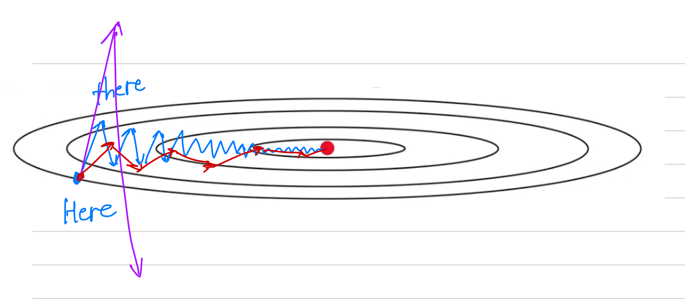
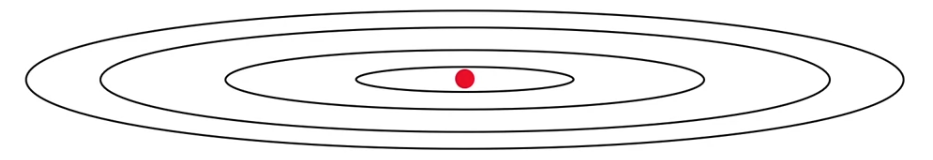
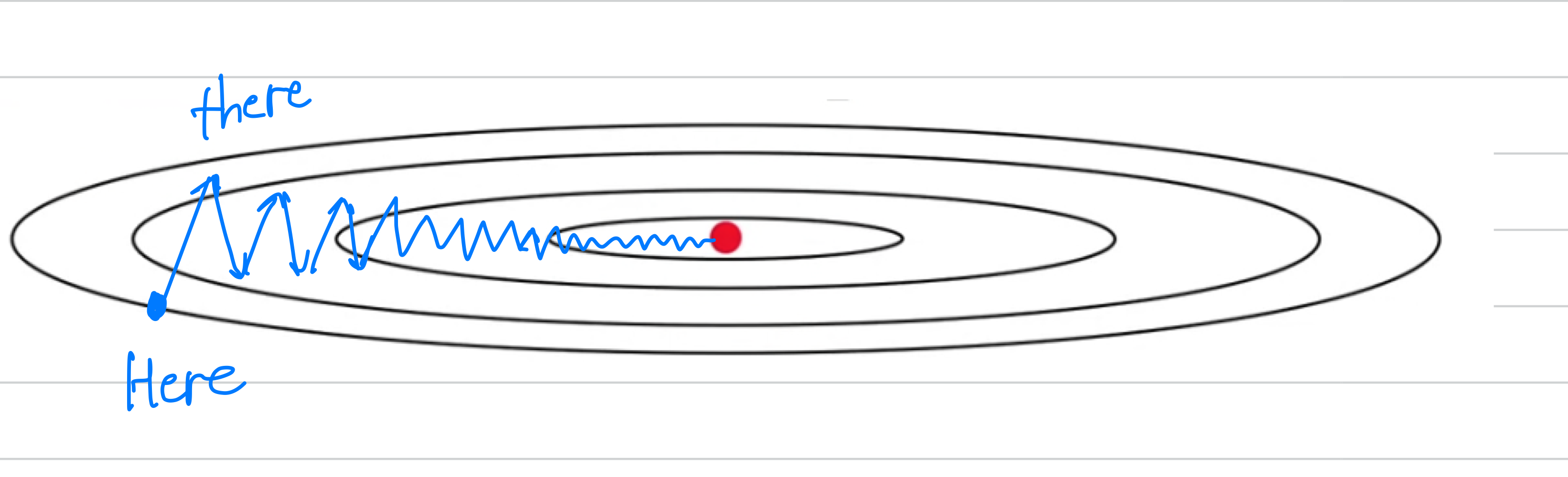
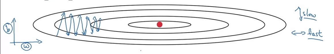
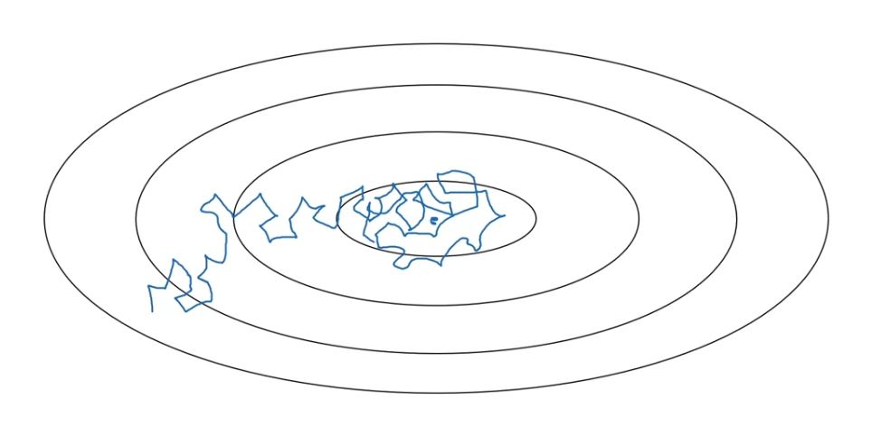
As a example let's say that you're trying to optimize a cost function
which has contours like this.
So the red dot denotes the position of the minimum.
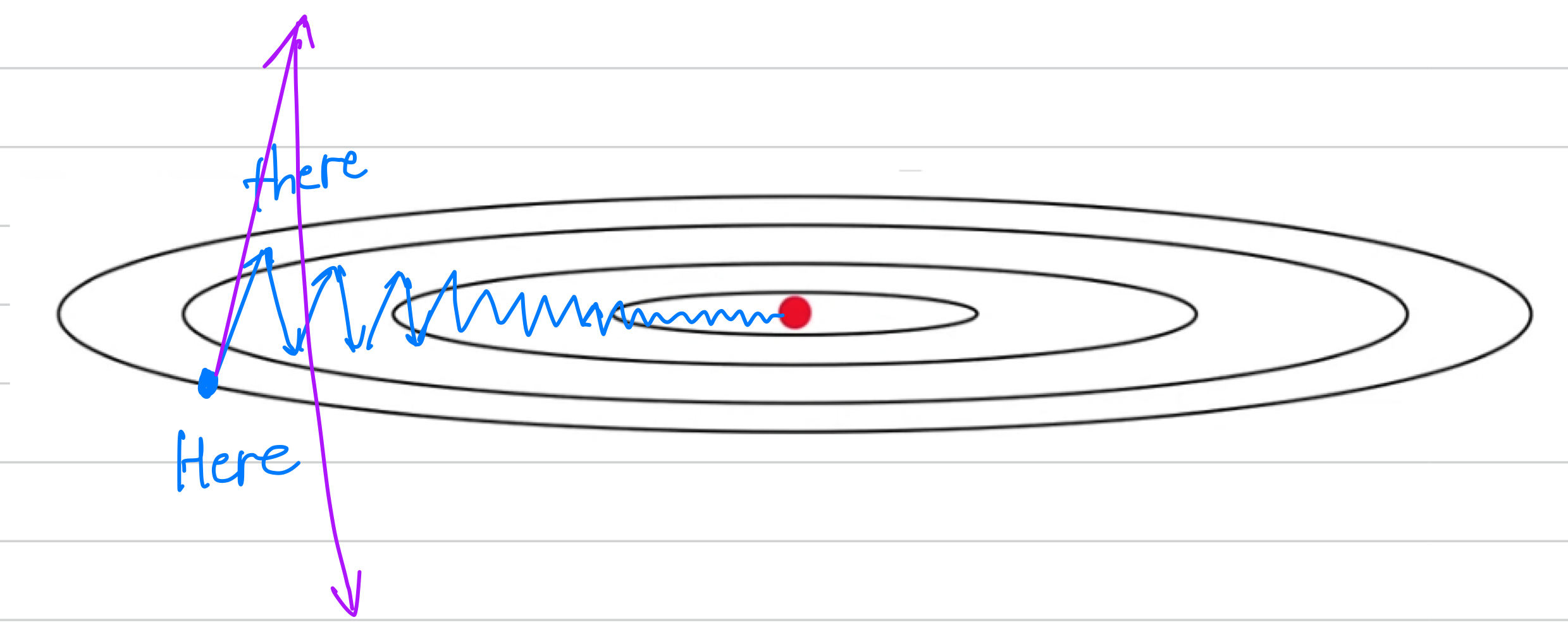
Maybe you start gradient descent here
and if you take one iteration of gradient descent maybe end up heading there.
And then another step, another step, and so on.
And you see that gradient descents will sort of take a lot of steps.
Just slowly oscillate toward the minimum.
And this up and down oscillations slows down gradient descsent and
prevents you from using a much larger learning rate.
In particular, if you were to use a much larger learning rate
you might end up overshooting and end up diverging like so.
And so the need to prevent the oscillations from getting too big forces you to use a learning rate that's not itself too large.
(따라서 osillation이 너무 커지는 것을 방지하기 위해 너무 크지 않은 learning rate를 사용할 필요가 있다.)
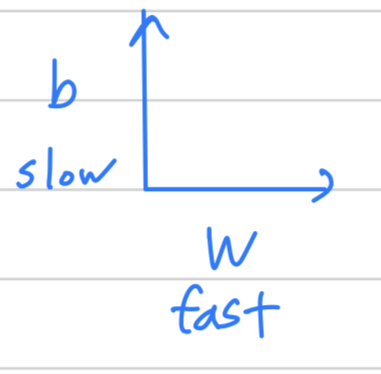
Another way of viewing this problem is that on the vertical axis.
You want your learning to be a bit slower, because you don't want those oscillations.
But on the horizontal axis, you want faster learning,
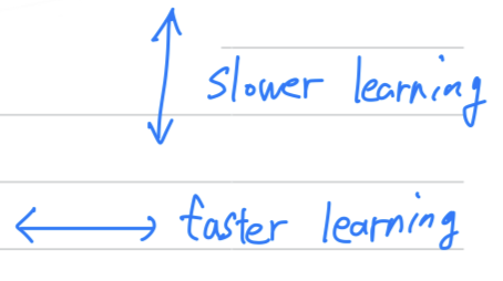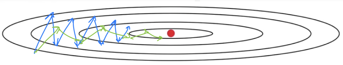
because you want it to aggressively move from left to right toward that minimum.So here's what you can do if you implement gradient descent with momentum.
So what this does is smooth out the steps of gradient descent.

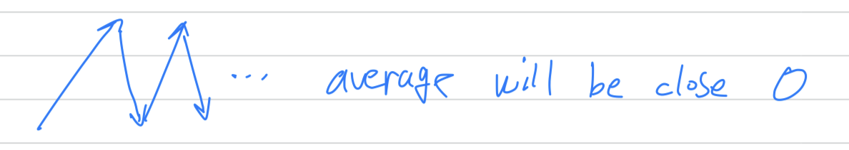
For example, let's say that in the last few derivatives you computed were this.
If you average out these gradients,
you find that the oscillations in the vertical direction will tend to average out to something close to $0$ .
So, in the vertical direction, where you want to slow things down,
this will average out positive and negative numbers, so the average will be close to $0$ .
Whereas, on the horizontal direction,
all the derivatives are pointing to the right of the horizontal direction,
so the average in the horizontal direction will still be pretty big.
So that's why with this algorithm, with a few iterations
you find that the gradient descent with momentum ends up eventually just taking steps that are much smaller oscillations in the vertical direction.
And so this allows your algorithm to take more straightforward path,
or to damp out the osciallations in this path to the minimum.
One intuition for this momentum is that
if you're trying to minimize the contours of a bowl.
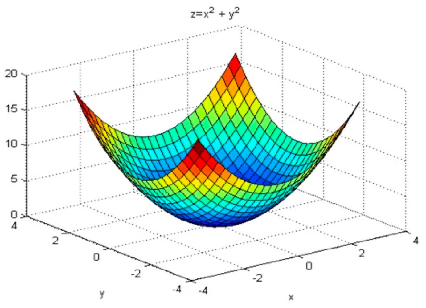They kind of minimize this type of bowl shaped function
then these derivates terms( $dW, db$ ) you can think of as providing acceleration
to a ball that you're rolling down hill.
And these momentum terms( $\beta V_{dW}, \beta B_{db }$ ) you can think of as representing the velocity.
And so imagine that you have a bowl,
and you take a ball and the derivative imparts acceleration to this little ball is rolling down this hill.
(작은 공을 가지고 있다고 가정하고, 미분이 이 작은 공을 언덕 아래로 굴러 내려가게 한다.)
And so it rolls faster and faster, because of acceleration.
And $\beta$ , because this number a little bit less than $1$ ,
displays a row of friction(마찰) and it prevents your ball from speeding up without limit.
(마찰력이 제공되어 속도가 무한으로 커지는 것을 방지해준다)
Now, your little ball can roll downhill and gain momentum(운동량),

Implementation details

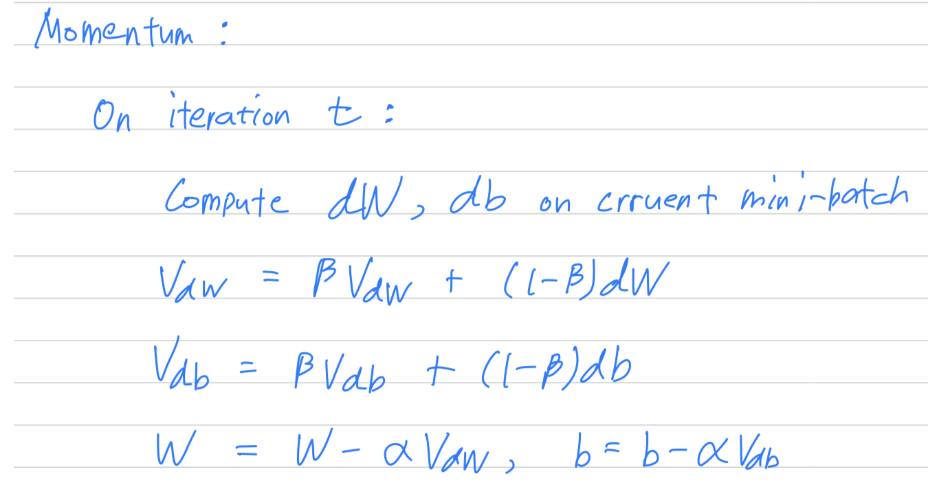
Let's look at some details on how you implement this.
You now have two hyperparameters
(learning rate : $\alpha$ , control your exponentially weighted average : $\beta$ )
The most common value for $\beta=0.9$
We're averaging over the last ten days temperature.
So it is averaging of the last ten iteration's gradients.
And in practice, $\beta=0.9$ works very well.

How about bias correction?
Do you want to take $\frac{V_{dW}}{1-\beta^t}$ ?
In practice, people don't usually do this beacuse after just ten iterations,
your moving average will have warmed up and is no longer a bias estimate.
(10 iteration만 돌려도 bias가 사라지기 때문에 bias correction을 굳이 하지 않아도 된다)

I just want to mention that if you read the literature on gradient descent with momentum
often you see it with this term( $(1-\beta)$ ) omitted,
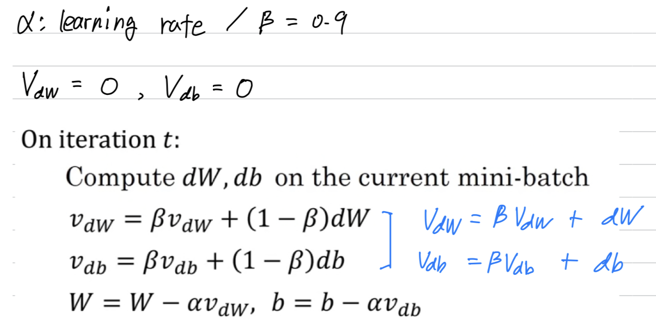And the net effect(최종 효과) of using this version in blue is that
$V_{dW}$ ends up being scaled by $\frac{1}{1-\beta}$ .
And so when you're performing gradient descent updates,
$\alpha$ just needs to change by a corresponding value of $\frac{1}{1-\beta}$ .

In practice, both of these will work just fine,
it just affects what's the best value of the learning rate $\alpha$ .
But i find that this particular formulation is a little less intuitive.
Because one impact of this is that if you end up tuning the hyperparameter $\beta$ ,
then this affects the scaling of $V_{dW}$ and $V_{db}$ as well.
And so you end up needing to return the learning rate, $\alpha$ , as well.
So i personally prefer the formulation that i have written on the left
rather than leaving out the $(1-\beta)$ term.
It's just at $\alpha$ , the learning rate would need to be tuned differently for these two different version.

RMSprop

You've seen how using momentum can speed up gradient descent.
There's another algorithm called RMSprop, which stands for root mean square prop,
that can also speed up gradient descent.
Recall our example from before,
that if you implement gradient descent,
you can end up with hugh oscillations in the vertical direction,
even while it's trying to make progress in the horizontal direction.
In order to provide intuition for this example, let's say that
the vertical axis is the parameter $b$ and horizontal axis is the parameter $w$ .
And so, you want to slow down the learning in the $b$ direction or in the vertical direction.
And speed up learning, or at least not slow it down in the horizontal direction.
(학습 속도를 높이기 위해 horizontal direction으로 속도를 늦추지 마라.)
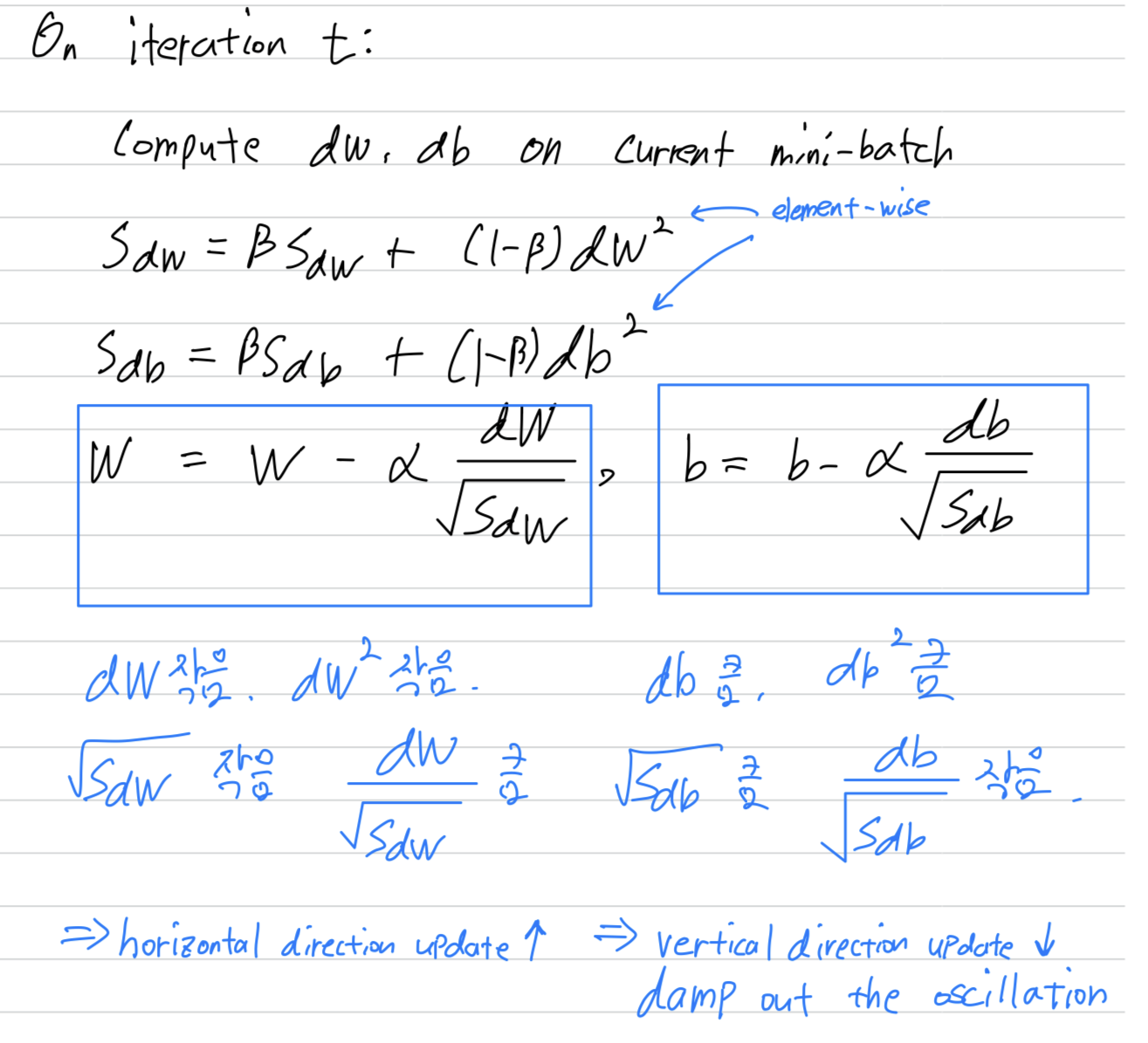
So this is what the RMSprop algorithm does to accomplish this.
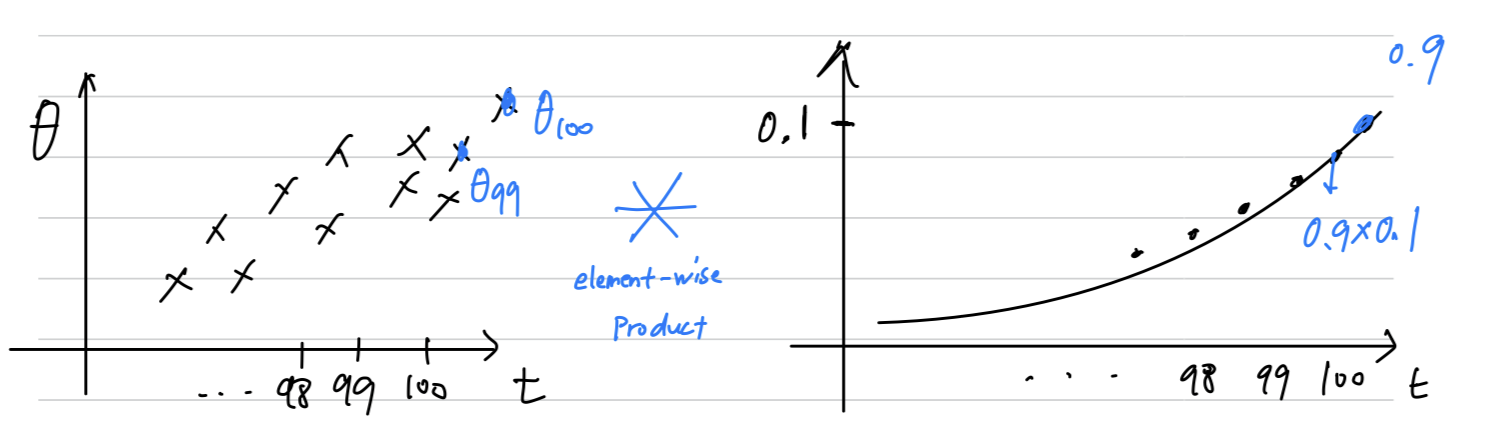
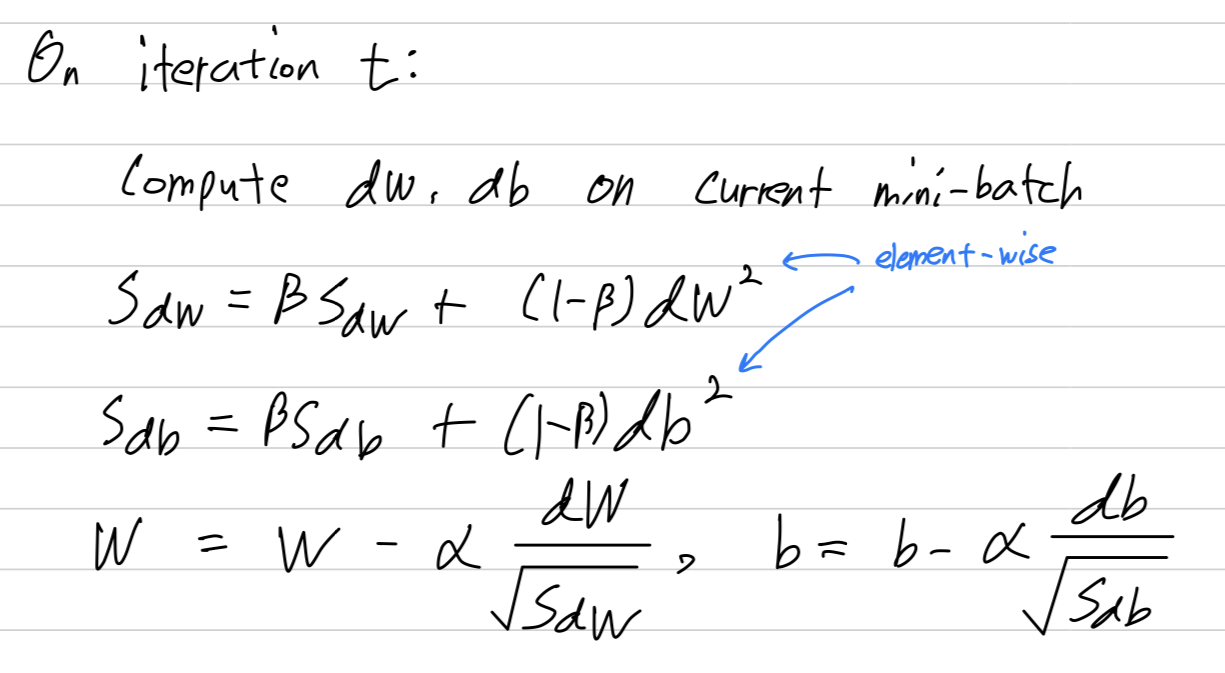That squaring operation is an element-wise squaring operation.
So what this is doing is keeping an exponentially weighted average of the squares of the derivatives.

So let's gain some intuition about how this works.
Recall that in the horizontal direction(= $w$ direction) we want learning to go pretty fast.
Whereas in the vertical direction(= $b$ direction) we want to slow down oscillations.
So with this terms $S_{dW}, S_{db}$ what we're hoping is that
$S_{dW}$ will be relatively small, so that we're dividing by relatively small number.
Whereas $S_{db}$ will be relatively large, so that we're dividing by relatively large number
in order to slow down the updates on a vertical dimension.

And indeed(실제로) if you look at these derivatives,
much larger in the vertical direction than in the horizontal direction.
So the slope is very large in the $b$ direction.
So with derivatives like this,
this is a very large $db$ and a relatively small $dW$ .
And so, $db^2$ will be relatively large, so $S_{db}$ will relatively large,
whereas compared to that $dW$ will be smaller, so $S_{dW}$ will be smaller.

So the net effect of this is that your updates in the vertical direction are divided by a much larger nubmer, and so that helps damp out the oscillations. Whereas the updates in the horizontal direction are divided by a smaller number. So the net impact of using RMSprop is that your updates will end up looking more like this.
And one effect of this is also that you can use a larger learning rate $\alpha$ .
and get faster learning without diverging in the vertical direction.
And also to make sure that your algorithm doesn't divide by $0$ .
What if square root of $S_{dW}$ is very close to $0$ .
Just to ensure numerical stability, when you implement this
in practice you add a very small $\epsilon$ to the denominator.
It doesn't matter what $\epsilon$ is used.
$10^{-8}$ would be a reasonable default.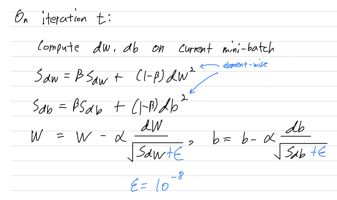

Adam optimization algorithm

During the history of deep learning,
many researchers sometimes proposed optimization algorithms
and show they work well in a few problems.
But thos optimization algorithms subsequently were shown not to really generalize that well to the wide range of neural networks you might want to train.

So over time, i think the deep learning community actually developed some amount of skepticism(회의감) about new optimization algorithms.
A lot of people felt that gradient descent with momentum really works well,
was difficult to propose things that work much better.

RMSprop and the Adam optimization algorithm, which we'll talk
is one of those rare algorithms that has really stood up(잘 알려진),
and has been shown to work well across a wide range of deep learning architectures.

So this one of the algorithms that i wouldn't hesitate to recommend you try
because many people have tried it and seeing it work well on many problems.
And the Adam optimization algorithm is basically taking
momentum and RMSprop, and putting them together.
(In the typical implemnetation of Adam, you do implement bias correction.)
Let's see how that works.
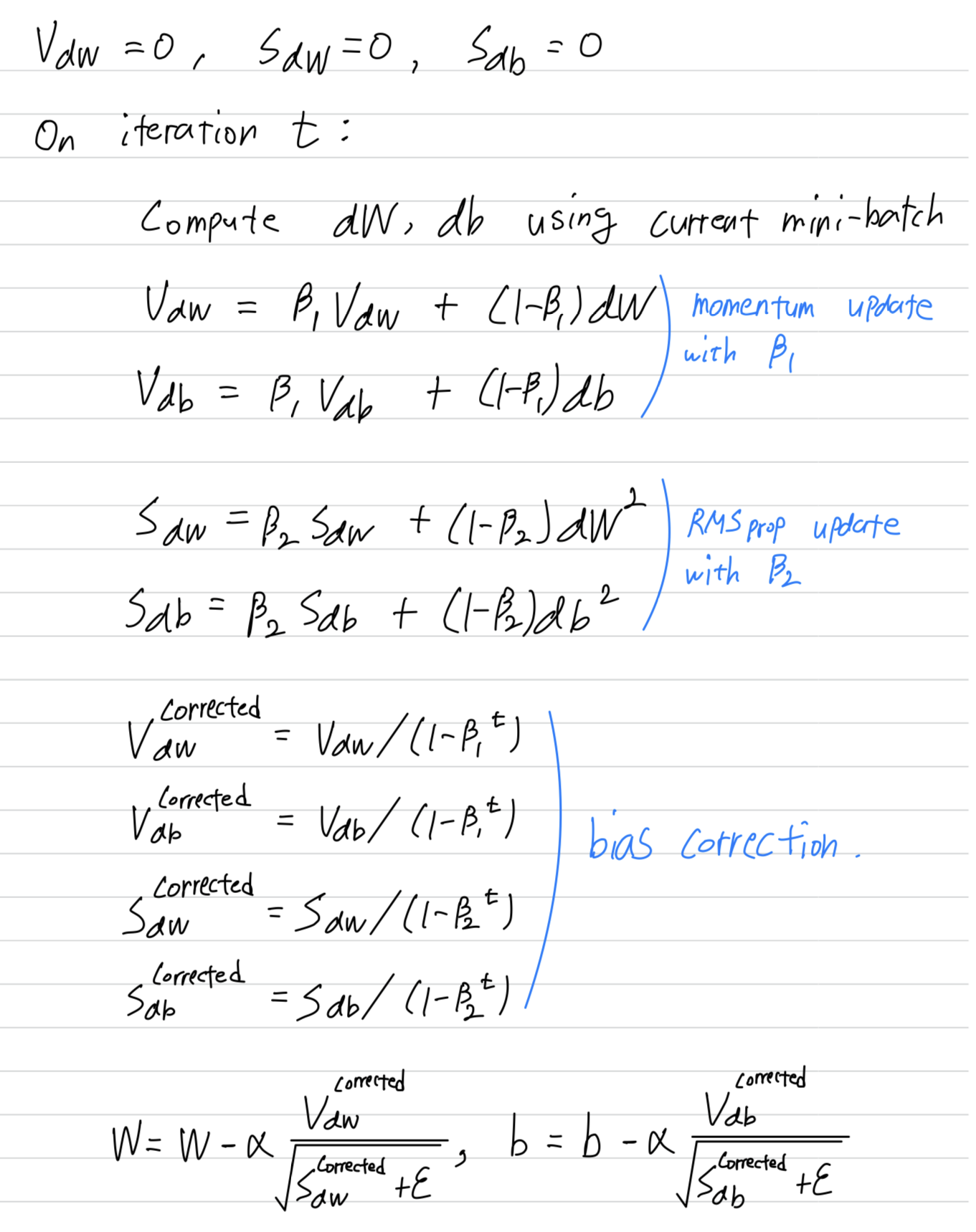These algorithm combines the effect of
gradient descent with momentum together with gradient descent with RMSprop.
This is commonly used learning algorithm that's proven to be very effective for many different neural networks of a very wide variety of architectures.

Hyperparameters choice

This algorithm has a number of hyperparameters.
- The learning rate hyperparameter $\alpha$ is still important and usually needs to be tuned,
  so you just have to try a range of values and see what works.
- We did a default(common) choice for $\beta_1 = 0.9$ ,
  so this is the moving weighted average of $dW, db$ .
  This is the momentum-like term.
- The hyperparameter for $\beta_2$ ,
  the author of the Adam paper inventors recommend $\beta_2=0.999$
  This is computing the moving weighted average of $dW^2, db^2$ .
  ➡️ You can also tune $\beta_1, \beta_2$ , but is not done that often among the practitioners i know.
- The choice of $\epsilon$ doesn't matter very much,
  but the authors of the Adam paper commend a $\epsilon=10^{-8}$
  but this parameter, you really don't need to set it,
  and it doesn't affect performance much at all.
So where does the term Adam come from?
Adam stands for adaptive moment estimation.
So $\beta_1$ is computing the mean of the derivatives.
This is called the first moment.
And $\beta_2$ is used to compute exponentially weighted average of the squares.
This is called the second moment.
That gives rise to the name adaptive moment estimation

Learning rate decay

One of the things that might help speed up your learning algorithm
is to slowly reduce your learning rate over time.
We call this learning rate decay.
Let's see how you can implement this.
Suppose you're implementing mini-batch gradient descents with a reasonably small mini-batch(64, 128),
then as you iterate, your steps will be a little bit noisy and it will tend towards this minimum over here,
but it won't exactly converge.
Your algorithm might just end up wandering around and never really converge
because you're using some fixed value for $\alpha$ and there's just some noise in your different mini-batches.
But if you were to slowly reduce your learning rate $\alpha$ ,
then during the initial phases, while your learning rate $\alpha$ is still large,
but then as $\alpha$ gets smaller, your steps you take will be slower and smaller,
and so you end up oscillating in a tighter region around this minimum rather than
wandering far away even as training goes on and on.
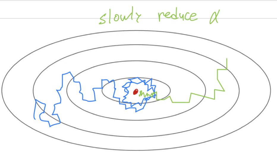The intuition behind slowly reducing $\alpha$ is that
maybe during the initial steps of learning, you could afford to take much bigger steps,
but then as learning approaches convergence, then having a slower learning rate allows you to take smaller steps.
Here's how you can implement learning rate deacy
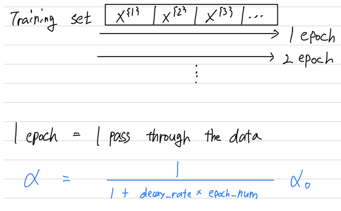Here's a concrete example.
If you take several epochs, so several passes through your data,
if $\alpha_0=0.2$ and the $decayRate=1$

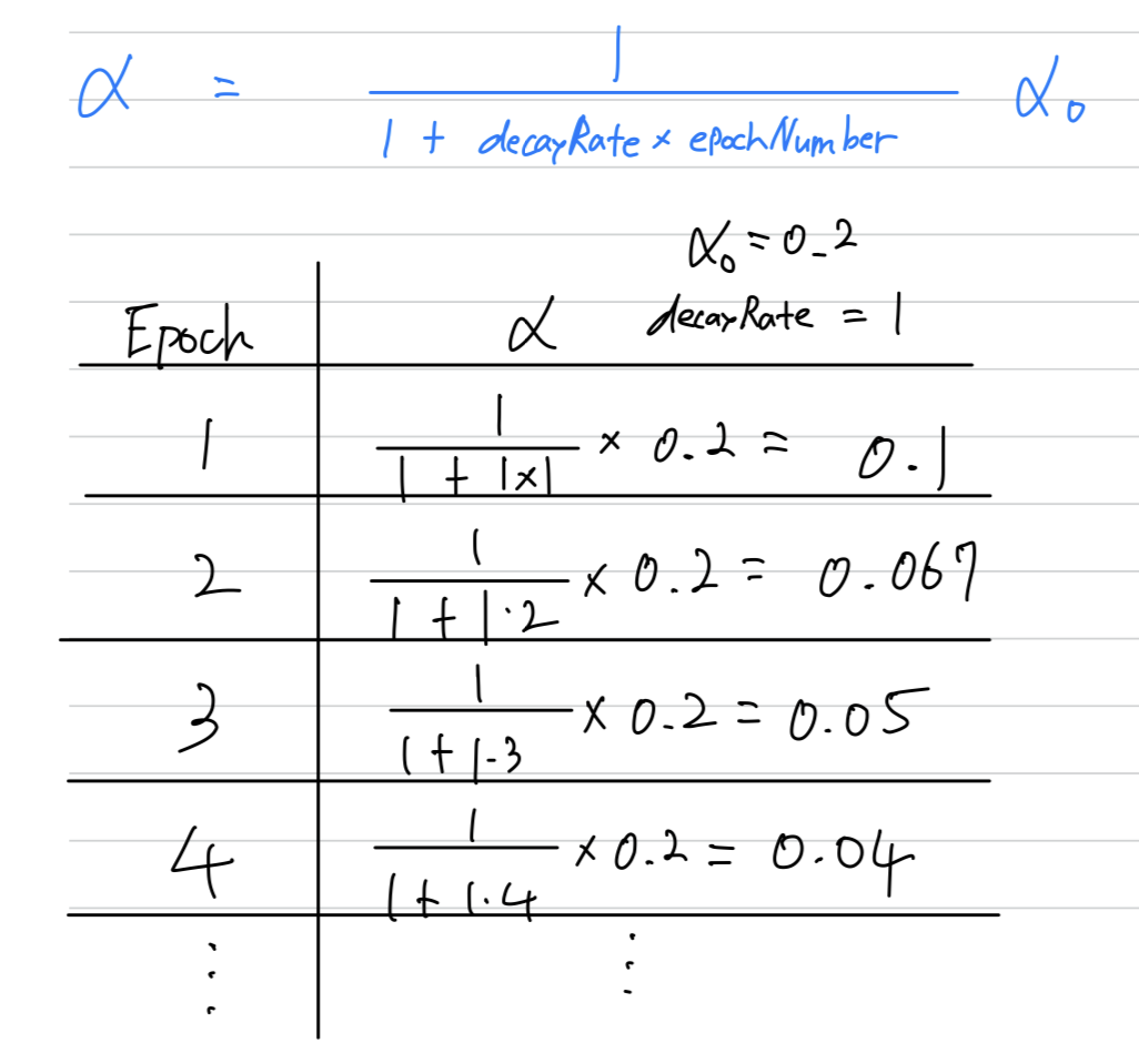
Other learning rate decay methods

Other than this formula for learning rate decay,
there are few other ways that people use.

Using some formula to govern how the learning rate( $\alpha$ ) changes over time.
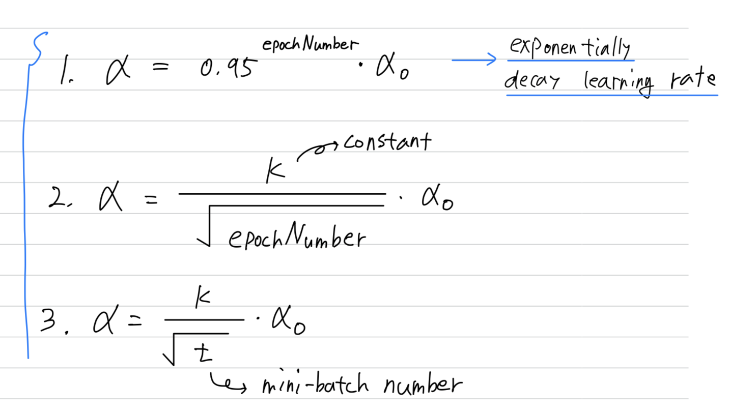
1. This is called exponentially decay learning rate where $\alpha$ is equal to some number less than $1$ such as $0.95$
  
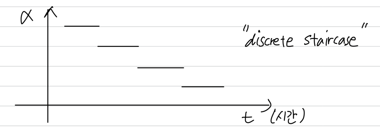
  Sometimes you also see people use a learning rate that
  decreases and discretes that where for some number of steps,
  you have some learning rate
  and then after a while, you decrease it by one-half, after a while, by one-half, and so,
  this is a discrete staircase.
One other thing that people sometimes do is manual decay(수작업).
If you're training just one model at a time,
what some people would do is just watch your model as it's training over a large number of days,
and they manually say "it looks like the learning rate slowed down, i'm going to decrease $\alpha$ a litlle bit."
Of course, this manually controlling $\alpha$ , tuning $\alpha$ by hand, hour-by-hour, day-by-day
works only if you're training only a small number of models,
but sometimes peoople do that as well.

Now, in case you're thinking
"Wow, there are a lot of hyperparameters, how do i select amongst all these different options?"
Don't worry about it for now, and next week we'll talk about how to systematically choose hyperparameters.

The Problem of Local Optima

In the early days of deep learning,
people used to worry a lot about the optimization algorithm getting stuck in bad local optima.
(좋지 않은 local optima에 갇히는 것에 대해 매우 불안해 했다.)
But as this theory of deep learning has advanced,
our understanding of local optima is also changing.
Let me show you how we now think about local optima and problems
in the optimization problem in deep learning.
This was a picture people used to have in mind when they worried about local optima.
In this picture, it looks like there are a lot of local optima in all those places.
And it'd be easy for gradient descent, or one of the other algorithms to get stuck
in a local optimum rather than find its way to a global optimum.
It turns out that if you are plotting a figure like this in two dimensions,
then it's easy to create plots like this with a lot of different local optima.
And these very low dimensional plots used to guide their intuition.
But his intuition isn't actually correct.
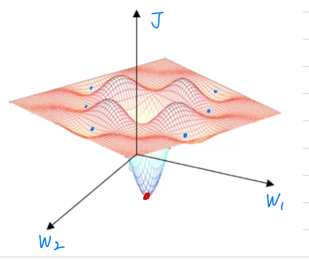It turns out if you create a neural network,
most points of zero gradients are not local optima like points like this.
Instead most points of zero gradient in a cost function are saddle points.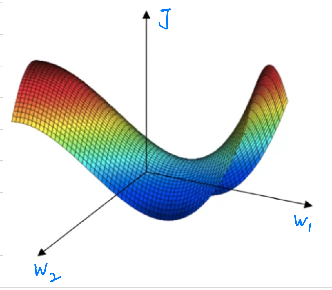But informally, a function of very high dimensional space,
if the gradient is zero, then in each direction it can either be a convex function or concave function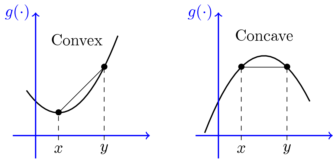And if you are in, say a 20,000 dimensional space,
then for it to be a local optima,
all 20,000 directions need to look like this(convex).
And so the chance of that happening is maybe very small, maybe $2^{-20,000}$ .
You're much more likely to get some directions where the curve bends up like so(saddle point).
So that's why in very high-dimensional spaces you're actually more likely to run into a saddle point, than the local optimum.
(예전에는 intuition을 위해 low-dimensional space에 대해 다뤘는데,
실제로 동작하는 algorithm은 high dimensional space이기 때문에
local optimum 문제보다 saddle point를 볼 가능성이 훨씬 더 높다.)
(convex, concave function들이 고차원적으로 섞여있다보니까 saddle point 형태로 나타남)

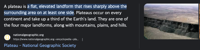
Problem of plateaus

If local optimum aren't a problem, then what is a problem?
It turns out that plateaus can really slow down learning
and a plateaus is a region where the derivative is close to zero for a long time.
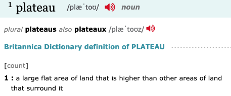
So if you're here, then gradient descents will move down the surface,
and because the gradient is zero or near zero.
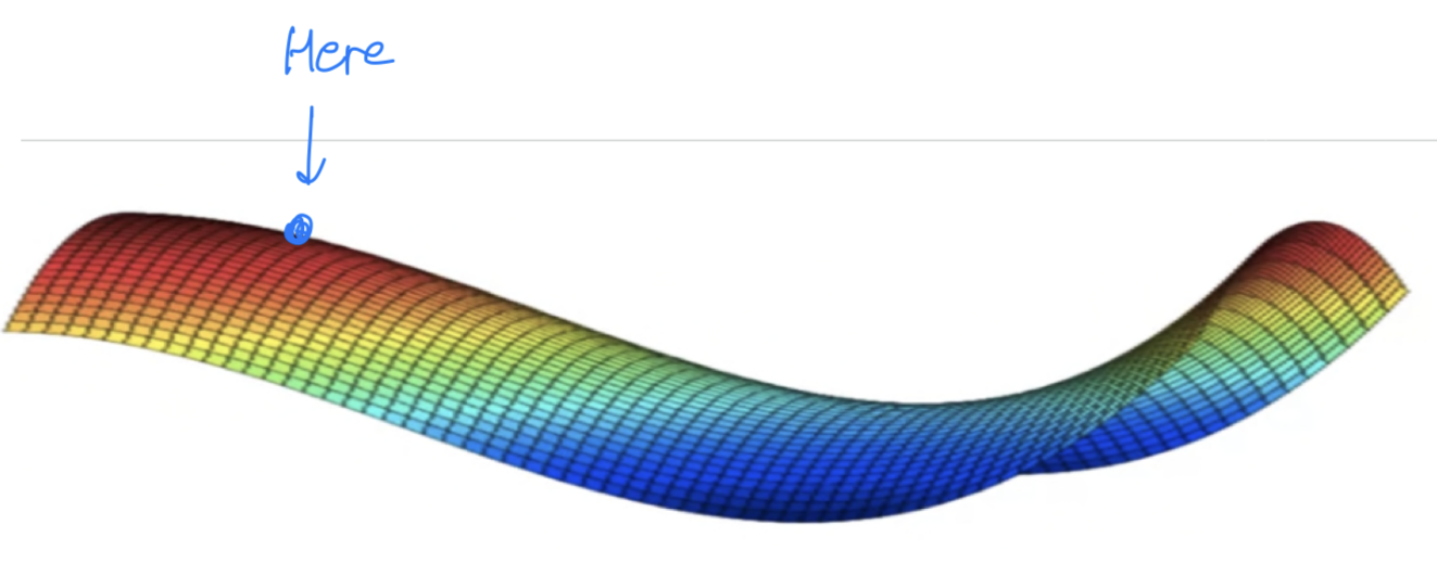
The surface is quite flat.
You can actually take a very long time to slowly find your way to maybe this point on the plateau,
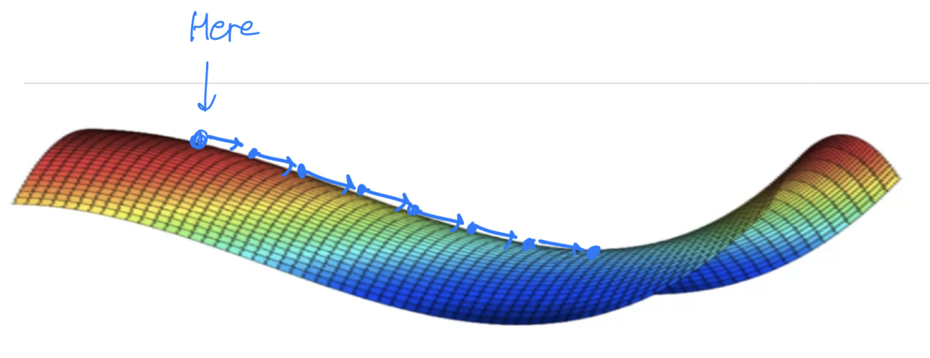and then because of random perturbation(혼란) of left or right
maybe then finally your algorithm can then find its way off the plateau.Let it take very long slope off before it's found its way here and they could get off this plateau.

You're actually pretty unlikely to get stuck in a bad local optima
so long as you're training a reasonably large neural network save a lot of parameters,
and the cost function $J$ is defined over a relatively high dimensional spaec.
(비교적 신경망이 큰 NN을 훈련하는 이상 local optima에 빠질 확률을 작으며,
cost function $J$ 는 비교적 high dimensional space에서 정의된다.)

Plateaus are a problem and you can actually make learning pretty slow.
And this is where algorithms like momentum or RMSprop or Adam
can really help your learning algorithm as well.

Seminar - discussion

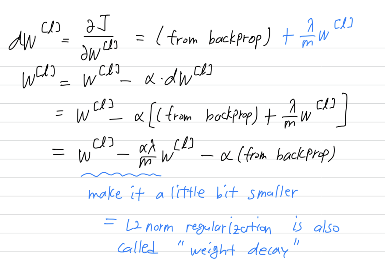
L2 Regularization의 효과는 Weight를 원래의 update보다 조금 더 크게 update를 하여 weight를 보다 작게 만든다.
W값들이 극단적으로 크거나 작은 값이 덜해지고, 어느정도 분포가 비슷해진다.
그럴수록 구별하는 능력이 떨어져서 overfitting을 방지할 수 있다.
momentum은 학습을 빠르게 만드는가?
exponentailly weighted average를 이용하여 parameter들을 update시키므로,
이전 $dW, db$ 값들의 누적된 계산을 통해 현재의 parameter값이 update된다.
vertical direction의 평균적인 계산은 0에 가까울 것이고,
horizontal direction의 평균적인 계산은 계속해서 오른쪽 방향을 가리키는 기울기가 될 것이므로 계속해서 가속화가 될 것이다.
따라서 vertical 방향으로의 oscillation은 줄어들고, horizontal 방향(=minimum이 있는 방향)으로의 speed는 점점 빨라질 것이다.
따라서 학습이 보다 빨라지게 된다.