Week 1 | Practical Aspects of Deep Learning | Setting up your Machine Learning Application
Train / Dev / Test sets
-
When training a neural network, you have to make a lot of decisions,
such as- the number of layers
- the number of hidden units
- learning rates
- activation functions
...
-
When you're starting on a new application,
it's almost impossible to correctly guess the right values for all of these,
and for other hyperparameter choices, on your first attempt. -
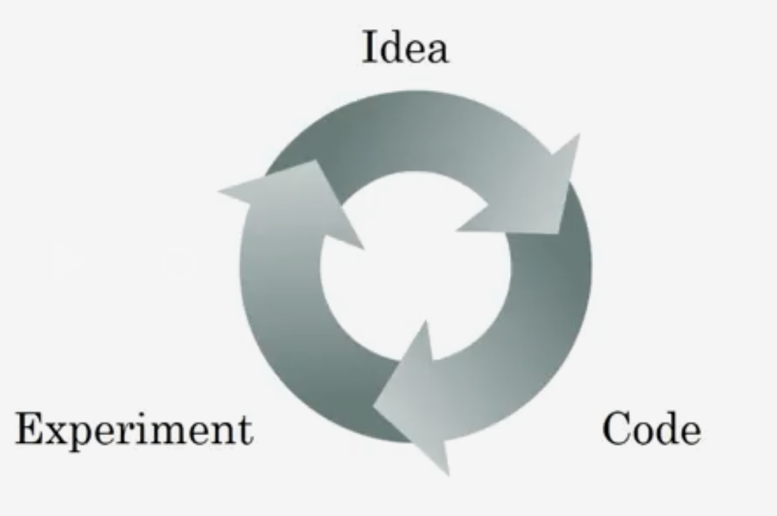
So, in practice, applied machine learning is a highly iterative process,
in which you often start with anidea,
such as you want to build a neural network of a certain number of layers,
a certain number of hidden units, maybe on certain data sets, and so on.
And then you just have tocodeit up and try it, by running your code.
You runexperimentand you get back a result that tells you how well this particular network, or this particular configuration works.
And based on the outcome,
you might then refine your ideas and change your choices and maybe keep iterating, in order to try to find a better and a better, neural network.
-
Today, deep learning has found great success in a lot of areas raning from natural language procesing(NLP), to computer vision, to speech recognition, to a lot of applications on also structured data.
And structured data includes everything from advertisements to web search,
which isn't just internet search engines.
It's also, for example, shopping websites. -
So what i'm seeing is that sometimes a researcher with a lot of experience in NLP
might try to do something in computer vision.
Or maybe a researcher with a lot of expereince in speech recognition
might jump in and try to do something advertising.
Or someone from sercurity might want to jump in and do something on logistics.
And what i've seen is that intuitions from one domain or from one application area
often do not transfer to other application areas.
And the best choices may depend on the amount of data you have,
the number of input features you have through your computer configuration and
whether you training on GPUs or CPUs.
-
Even very experienced deep learning people find it almost impossible to correctly guess
the best choice of hyperparameters the very first time.
And so today, applied deep learning is a veryiterative process
where you just have to go around this cycle many times to hopefully find a good choice of network for your application.
Train / dev / test sets
So one of the things that determine how quickly you can make progress
is how efficiently you can go around this cycle.
And setting up your data sets well, in terms of your train, development and test sets can mke you much more efficient at that.
-
So if this is your training data,
Then traditionally,
you might take all the data you have and carve off
some portion of it to be yourtraining set,
some portion of it to be yourhold-out cross validation set == development set == dev set,
some final portion of it to be yourtest set.
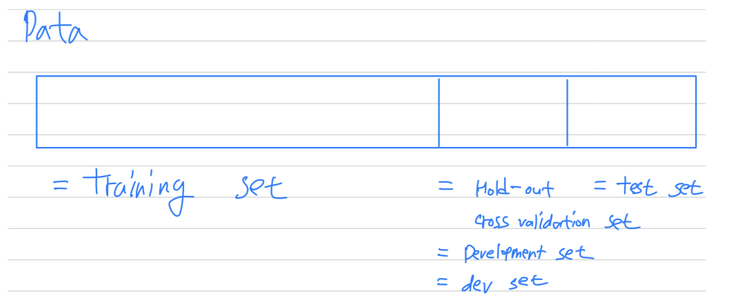
- And so the workflow is that you keep on training algorithm on your
training set - And use your
dev setor yourhold-out cross validation set
to see which of many different models performs best on your dev set, - And than after having done this long enough,
when you have a final model that you want to evaluate,
you can take the best model you have found and evaluate it on yourtest setin order to get an unbiased estimate of how well your algorithm is doing.
- And so the workflow is that you keep on training algorithm on your
-
So
in previous era of machine learning, it was common practice to take all your data and
split it according to maybe a 70/30% in terms of people talk about the 70/30 train test splits if you don't have an explicit dev set.
Or maybe a 60/20/20% splits, in terms of 60% train, 20% dev and 20% test.
And several years ago, this was widely considered best practice in machine learning.
If you have here maybe 100 exampels in total, maybe 1,000 examples in total, maybe after 10,000 examples, these sorts of ratios were perfectly reasonable rules of thumb. -
But
in the modern big data era,
the trend is that your dev and test sets have been becoming a much smaller percentage of the total.-
Because remember,
the goal of the dev set or the development setis that you're going to test different algorithms on it and see which algorithm works better.
So the dev set just needs to be big enough for you to evaluate, say, two different algorithm choices or ten different algorithm choices and quickly decide which one is doing better.
And you might not need a whole 20% of your data for that(dev set).
So, for example, if you have a million trainin examples,
you might decide that just having 10,000 examples in your dev set is more than enough to evaluate which one or two algorithms does better. -
And in a similar vein,
the main goal of your test setis given your final classifier to give you a pretty confident estimate of how well it's doing.
And again, if you have a million exmamples,
maybe you might decide that 10,000 examples is more than enough in order to evaluate a single classifier and give you a good estimate of how well it's doing. -
So, in this example, where you have a 1,000,000 examples,
if you need just 10,000 for you dev and 10,000 for your test,
your ratio will be more like 1% of million, 1% of million,
so you'll have 98% train, 1% dev, 1% test.
-
-
And i've also seen application where,
if you have even more than a million example,
you might end up with, 99.5% train and 0.25% dev, 0.25% test.
Or maybe a 0.4% dev, 0.1% test.
So just to recap, when setting up your machine learning problem,
I'll often set it up into atrain, dev and test sets,
andif you have a relatively small dataset,
these traditional ratios might be okay. (70/30 or 60/20/20)
Butif you have a much larger data set,
it's also fine to set your dev and test sets to be much smaller than
your 20% or even 10% of your data. (like 98% train, 1% dev, 1% test)
Mismatched train/test distribution
-
Let's say you're building an app that lets users upload a lot of pictures
and your goal is to find pictures of cats in order to show your users.- Maybe your training set comes from cat pictures downloaded off the internet
➡️ turns out a lot of webpages have very high resolution, very professional, very nicely framed pictures of cats.
- but your dev and test sets might comprise cat pictures from users using your app.
- maybe your users are uploading, blurrier, lower resolution image just taken with a cell phone camera in a more casual condition.
- Maybe your training set comes from cat pictures downloaded off the internet
-
And so these two distributions of data may be different.
The rule of thumb he'd encourage you to follow, in this case,
is to make sure that the dev and test sets come from the same distribution. -
Finally, it might be okay to not have a test set.
Remember, the goal of the test set is to give you a unbiased estimate
of the performance of your final network, of the network that you selected.
But if you don't need that unbiased estimate, then it might be okay to not have a test set.
So what you do, if you have only a dev set but not a test set,
is you train on the training set and then you try different model architectures.
Evaluate them on the dev set, and then use that to iterate and try to get to a good model.
Because you've fit your data to the dev set,
this no longer gives you an unbiased estimate of performance.
-
In the machine learning world, when you have just a train and a dev set but no serparte test set,
most people will call the dev set the test set.
But what they actually end up doing is using the test set as a hold-out cross validation set.
Which maybe isn't completely a great use of terminology,
because they're then overfitting to the test set.
Even though i think calling it a train and devlopment set would be more correct terminology.
And this is actually okay practice if you don't need a completely unbiased estimated of the performance of you algorithm.
So when the team tells you that they have only a train and a test set,
i would just be cautions and think, do they really have a train//dev set?
Because they're overfitting to the test set.
Bias and Variance
-
Bias and Variance is one of those concepts that's easily learned but difficult to master.
-
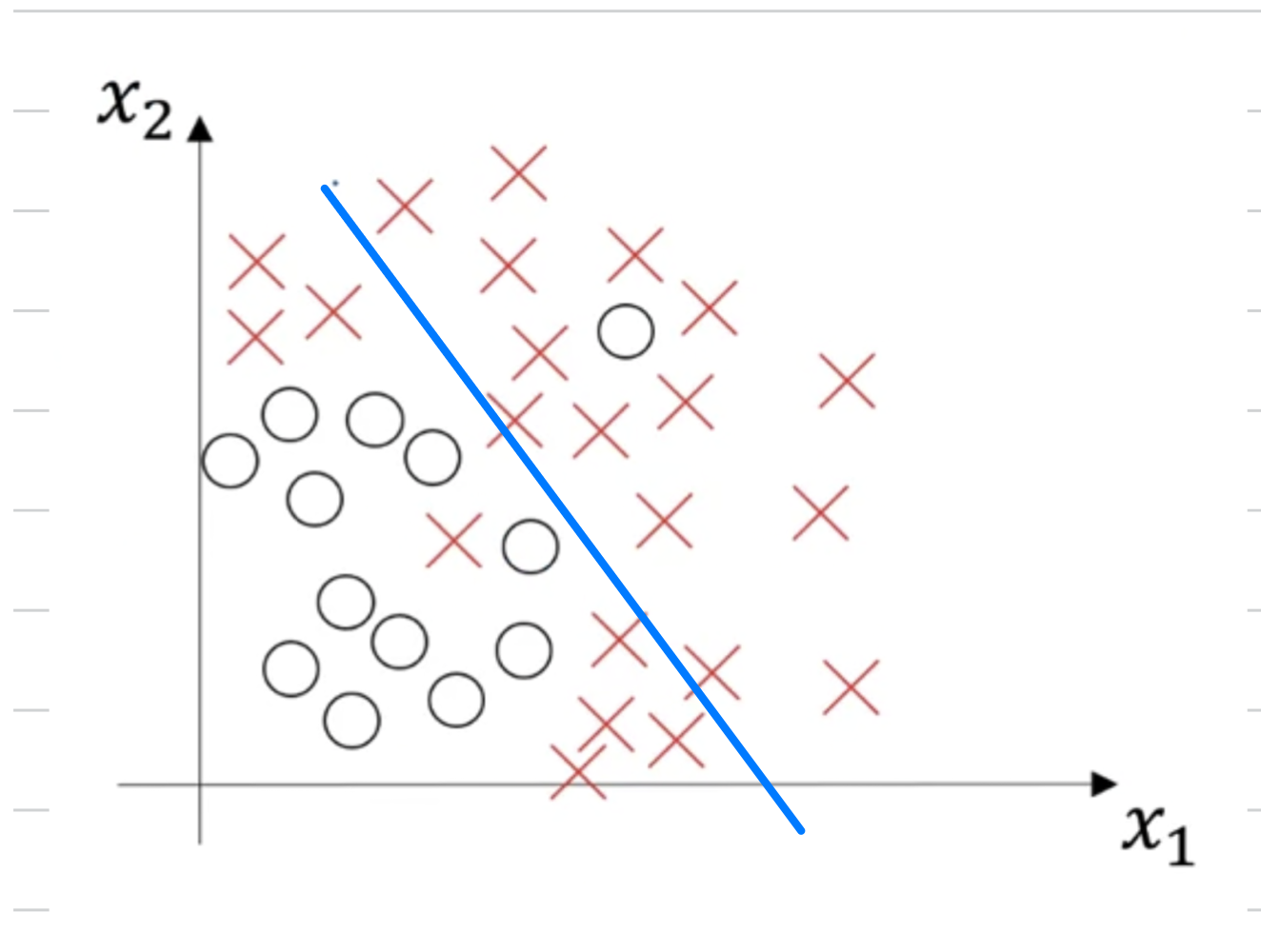
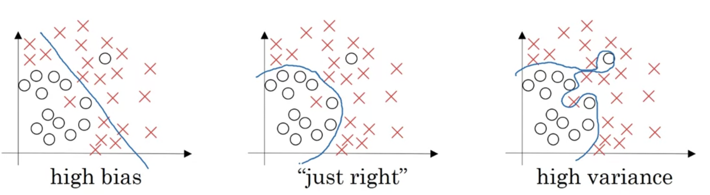
Let's see the data set that looks like this.
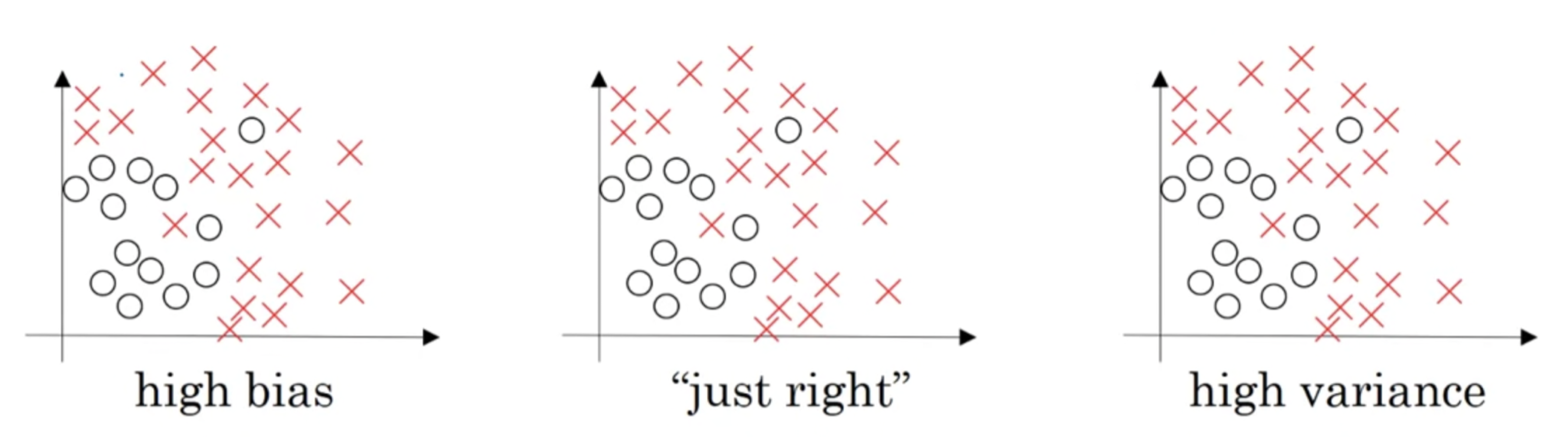
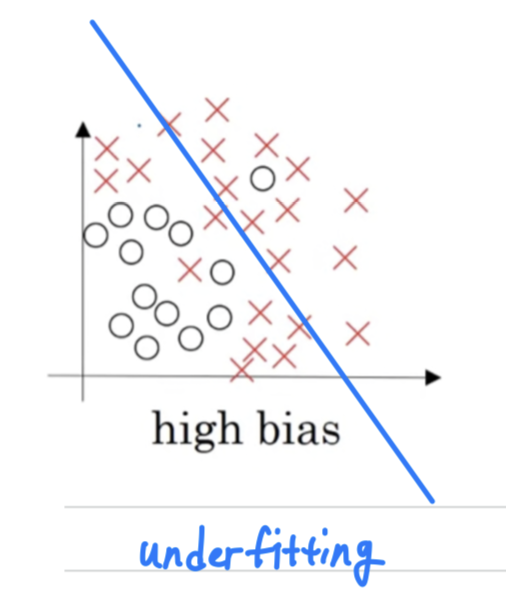
- If you fit a straight line to the data, maybe get a logistic regression fit to that.
This is not a very good fit to the data, and so this is a class of high bias.
So we say that this is underfitting the data.
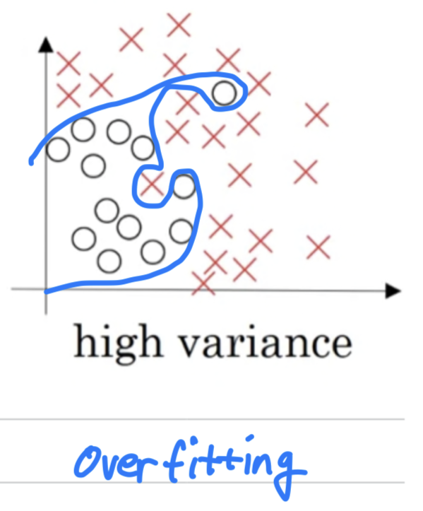
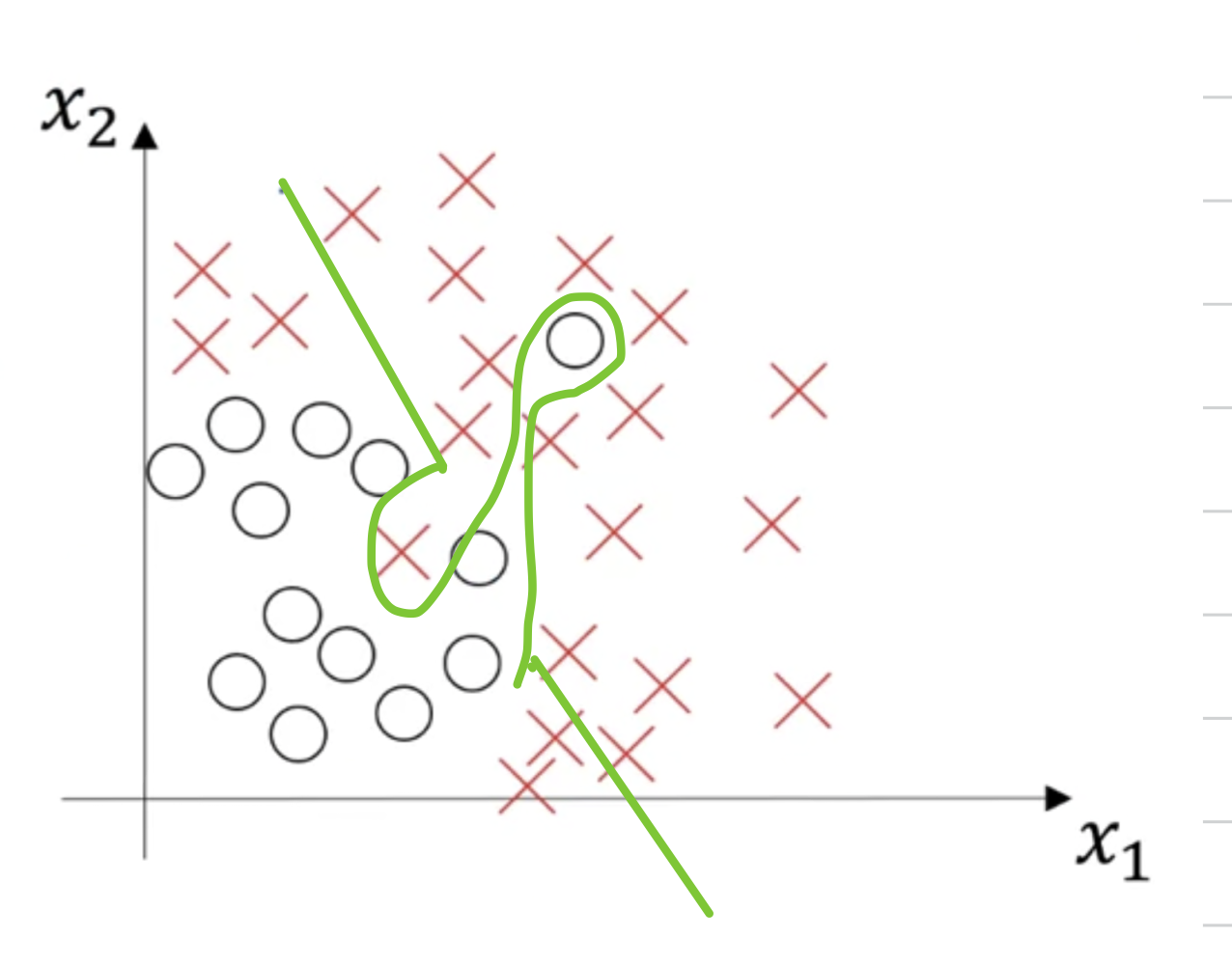
- On the opposite end,
if you fit an incredibly complex classifier,
maybe a deep neural network or a neural network with a lot of hidden units,
maybe you can fit the data perfectly
but that doesn't look like a great fit either.
So there's a classifier of high variance and this is overfitting the data.
- And there might be some classifier in between with a medium level of complexity,
maybe fits the curve like that.
That looks like a much more reasonable fit to the data.
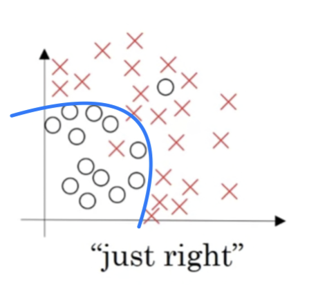
- If you fit a straight line to the data, maybe get a logistic regression fit to that.
-
So in a 2D example like this, with just two features,
you can plot the data and visualize bias and variance.
In high dimensional problems,
you can't plot the data and visualize divisoin boundary. -
So continuing our example of cat picture classification
where that's a positive example and that's a negative example.
The two key numbers to look at, to understand bias and variance,
will be the train set error and the dev set or the development set error.-
So for the sake of argument(논점을 위해서),
let's say that you're recognizing cats in pictures, is something that people can do nearly perfectly.
And so, let's say, your training set error 1% and your dev set error is 11%.
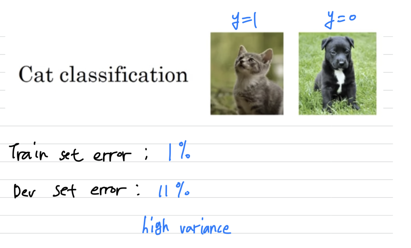
This looks like you might have overfit the trainin set,
that somehow you're not generalizing well to this hold-out cross validation set.
And so if you have an example like this,
we would say this is overfitting the data and this has high variance.
So by looking at the training set error and the development set error,
you would be able to render a diagnosis of your algorithm having high variance. -
Now, let's say, that you measure your training set and your dev set error, and you get a different result.
Let's say that your training set error is 15% and your dev set error is 16%.
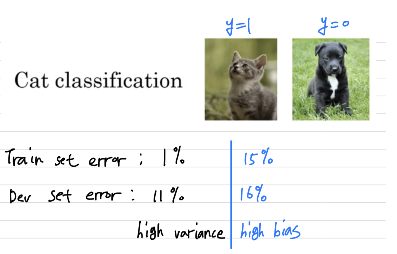 In this case, assuming that humans achieve, roughly 0% error,
then it looks like algorithm is not even doing very well on the training set.
So if it's not even fitting the training data as een that well,
then this is underfitting the data and so this algorithm has high bias.
So this algorithm has a problem of high bias,
beacuse it was not even fitting the training set. -
Now, here's another example.
Let's say that you have 15% training set error, so that's pretty high bias,
but when you evaluate to the dev set it does even worse, maybe it does, 30%.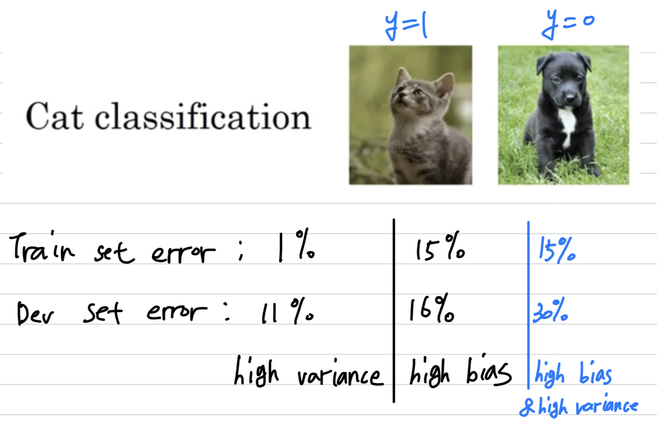 In this case, I would diagnose this algorithm as having high bias,
because it's not doing that well on the training set,
And high variance. -
And one last exapmle,
if you have 0.5% training set error and 1% dev set error,
then maybe our users are quite happy,
that you have a cat classifer with only 1% error.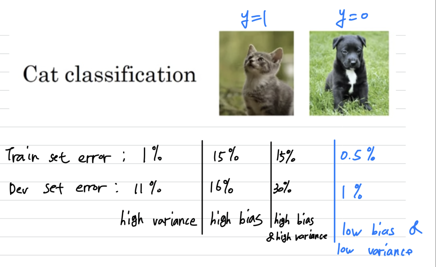 then this will have low bias and low variance.
-
High bias and High variance
-
What does high bias and high variance look like?
-
we said that a classifier like this,
a linear classifier has high bias
because it underfits the data.
-
So this would be a classifier that is mostly linear,
and therefore underfits the data
but if somehow your classifier does some weird things,
then it's actually overfitting parts of the data as well.
Where it has high bias, becuase, by being a mostly linear classifier, it's just not fitting, quadratic line shape that well.
But by having too much flexibility in the middle, it overfits those two examples as well.
So this classifier kind of has high bias, because it was mostly linear but you need maybe a curve function or quadratic function.
And it has high variance, because it had too much flexibility to fit, those two mislabel or those aligned examles in the middle as well.
So to summarize, you've seen how by looking at your algorithm's error on the training set and your algorithm's error on the dev set,
you can try to diagnose whether it has problems of high bias, or high variance, or maybe both, or maybe neither.
And depending on whether your algorithm suffers from bias or variance,
it turns out that there are different things you could try.
So there is a basic recipe for Machine learning that let's you more systematically try to improve your algorithm,
depending on whether it has high bias or high variance issues.
Basic Recipe for Machine Learning
-
In the previous video,
you saw how looking at training error and dev error can help you diagnose
whether your algorithm has a bias aor a variance problem, or maybe both. -
It turns out that this information that lets you much more systematically ,
using what they call a basic receipe for machine learning and let's you much more systematically go about improving your algorithm's performance.
- When training a neural network, here's a basic recipe i will use.
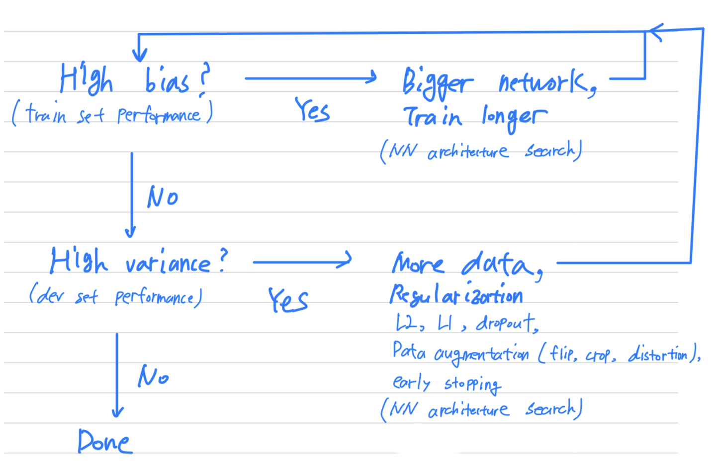
- After having trained in an initial model, I will first ask
does your algorithm have high bias?
And so, to try and evaluate if there is high bias,
you should look at the training set or the training data performance.
And so, if it does have high bias, does not even fitting in the training set that well,
some things you could try would be to try pick a network such as more hidden layers or more hidden untis, or you could train it longer.
I would try these things until I can at least get rid of teh bias problems.
(And usually, if you have a big enough network,
you should usually be able to fit the training data well.) - Once you've reduce bias to acceptable amounts, i will then ask
do you have a variance problem?
(= Are you able to generalize, from a pretty good training set performance, to having a pretty good dev set performance?)
And so to evaluate that i would look at dev set performance.
And if you have high variance,
best way to solve a high variance problem is to get more data if you can get it.
But sometimes you can't get more data.
You could try regularization which we'll talk about in the next video to try to reduce overfitting.
And then also, again, sometimes you just have to try it.
But if you can find a more appropriate neural network architecture,
sometimes that can reduce your variance problem as well as reduce your bias problem.
I try these things and i kind of keep going back, until, hopefully, you find something with both low bias and low variance whereupon you would be done.
- So a couple of points to notice.
- First is that depending on whether you have high bias or high variance,
the set of things you should try could be quite different.
So i'll ususally use the training dev set to try to diagnose if you have a bias or variance problem,
and then use that to select the appropriate subset of things to try.
So, for example, if you actually have a high bias problem, getting more training data is actually not going to help.
So being clear on how much of a bias problem or variance problem or both,
can help you focus on selecting the most useful things to try. - Second, in the earlier era of machine learning,
there used to be a lot of discussion on what is called the bias variance tradeoff.
And the reason for that was that, for a lot of the things you could try,
you could increase bias and reduce variance, or reduc ebias and increase variance,
But back in the pre-deep learning era,
we didn't have many tools, we didn't have as many tools that just reduce bisa,
or that just reduce variance without hurting the other one.
But in the modern deep learning, big data era,
so long as you can keep training a bigger network,
and so long as you can keep getting more data,
which isn't always the case for either of these,
but if that's the case, then getting a bigger network almost always just reduces your bias,
without necessarily hurting your variance,
so long as you regularize appropriately.
- First is that depending on whether you have high bias or high variance,
Regularization
If you suspect your neural network you is overfitting your data, that is, you have a high variance problem,
one of the first things you should try is probably regularization.
Logistic regression
-
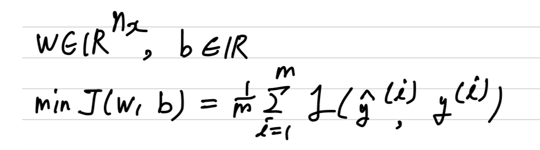
Let's develop these ideas using logistic regression.
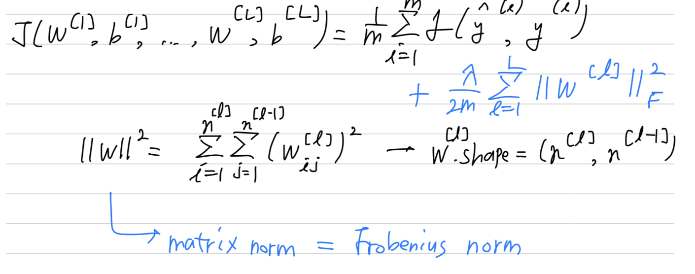
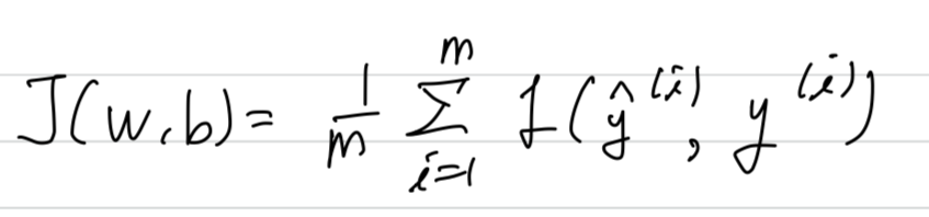
Recall that for logistic regression, you try to minimize the cost function ,
which is defined as this cost function.
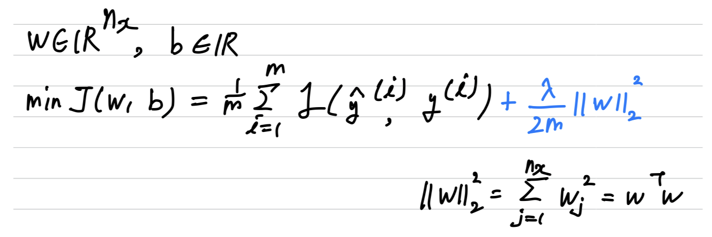
 And so, to add regularization to logistic regression, what you do is add to it
, which is called the regularization parameter.
And this is calledL2 regularization
-
Now, why do you regularize just the parameter ?
Why don't we add something here, you know, about as well?
Because if you look at your parameters, is usually a pretty high dimensional parameter vector,
especially with a high variance problem.
Maybe just has a lot of parameters, so you aren't fitting all the parameters well,
whereas is just a single number.
So almost all the parameters are in rather than .
And if you add this last term, in practice, it won't make much of a difference,
because is just one parameter over a very large number of parameters. -
And that's when you add, instead of L2 norm, this is called the L1 norm of the parameter vector .
If you useL1 regularization, then will end up being sparse.
And what that means is that the vector will have a lot of zeros in it.
And some people say that this can help with compressing the model,
because the set of parameters are zero, then you need less memory to store the model.
Although, i find that, in practice, L1 regularization, to make your model sparse, helps only a little bit.
So i don't think it's used that much, at least not for the purpose of compressing your model.
And when people train your networks, L2 regularization is just used much, much more often.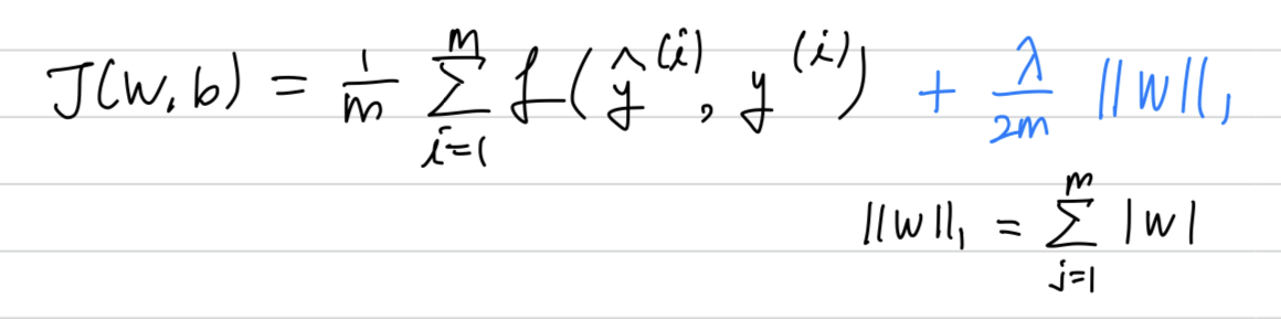
- is called `the regularization parameter.
And usually, you set this using your development set.
When you try a variety of values and see what does the best,
in terms of trading off between doing well in your training set versus
also setting that two norm of your paramters to be small,
which helps prevent overfitting,
So is another hyper parameter that you might have to tune.
And by the way, for the programming exercises,
is a reserved keyword in the Python programming language.
So in the programming exercise, we will have lambd without the 'a'
Neural network
-
In a neural network, you have a cost function that's a function of all of your parameters ()
-
So how do you implement gradient descent with this?
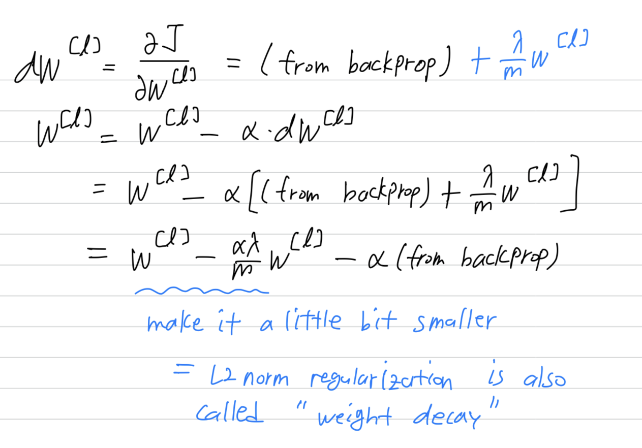 And it's for this reason that regularization is sometimes also called
 weight decay.
Why regularization reduces overfitting
intuition 1
-
So, recall that our high bias, just right, high variance pictures from our earlier video had looked somthing like this.
-
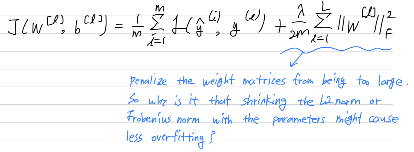
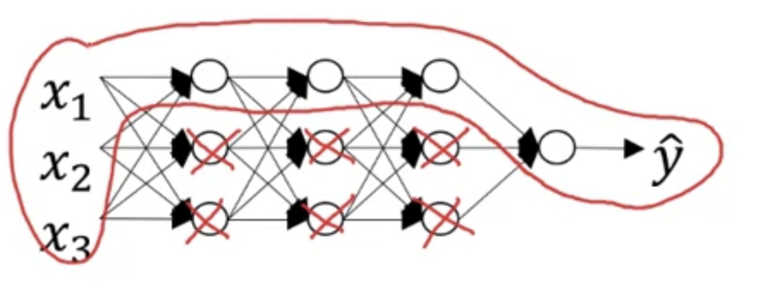
One piece of intuition is that if you crank your regularization to be really, really big,
that'll be really incentivized to set the weight matrices, , to be reasonably close to zero.
So one piece of intuition is maybe it'll set the weight to be so close to zero for
a lot of hidden units that's basically zeroing out a lot of the impact of these hidden units.
And if that's the case, then, this much simplified neural network becomes a much smaller neural network.
In fact, it is almost like a logistic regression unit but stacked multiple layers deep.
And so that will take you from this overfitting case, much closer to the "high bias" case.
Hopefully, there'll be an intermediate value of that results in the closer to the "just right" case.
intuition 2
- Here's another attempt at additional intuition for why regularization helps preven overfitting.
And for this, i'm going to assume that we're using the activation function.
so if takes on only a smallish range of parameters, then you're just using the linear region of the function.
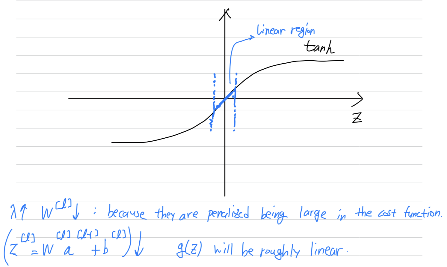 So every layer will be roughly linear as if it is just linear regression.
So just to summarize,
if the regularizatino parameters are very large,
the parameters very small so will be relatively small,
but so is relatively small, and so the activation function if it's tanh, will be relatively linear.
And so whole neural network will be computing something not too far from a big linear function,
which is therefore, pretty simple function, rather than a very complex highly non-linear function.
And so, is also much less able to overfit.
Dropout regularization
-
In addition to L2 regularization, another powerful regularization technique is called
dropout. -
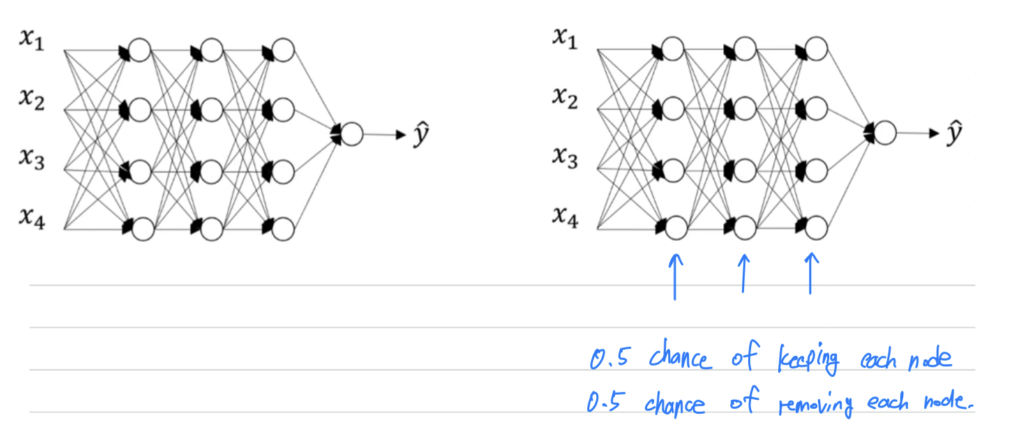
With dropout, what we're going to do is go through each of the layers of the network and
set network probability of eliminating a node in neural network.
Let's say that for each these layers, we're going to for each node,
toss a coin and have a 0.5 chance of keeping each node and 0.5 chance of removing each node.
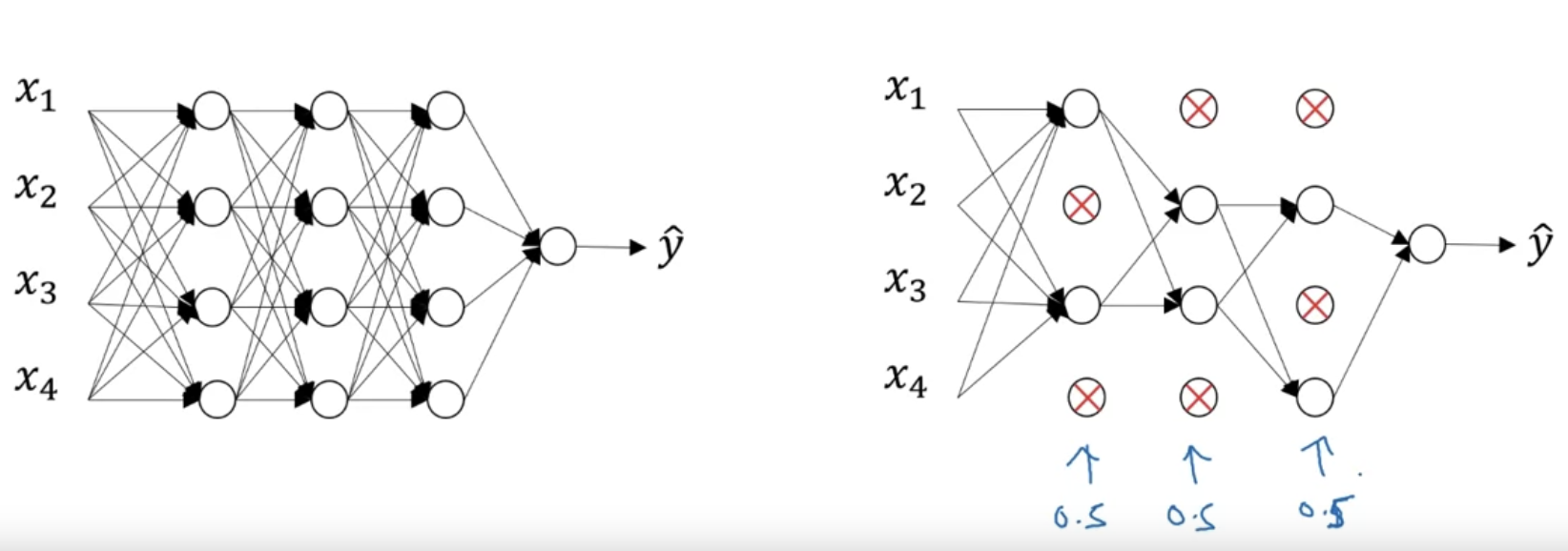
-
So, after the coin tosses, maybe we'll decide to eliminate those nodes,
then what you do is actually remove all the ingoing, outgoing things from that nodes as well.
So you end up with a much smaller, really much diminished network.
And then you do back propagation training.
There's one example on this much diminished network.
-
And then on different examples,
you would toss a set of coins again and
keep a different set of nodes and then dropout or eliminate different set of nodes.
And so for each training example, you would train it using one of these neural based networks.
So, maybe it seems like a slightly crazy technique. They just go around coding those are random,
but this actually works.
Implementing dropout("Inverted dropout")
-
There are few ways of implementing dropout.
I'm going to show you the most common one, which is technique calledinverted dropout. -
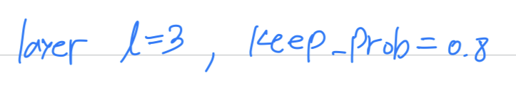
For the sake of completeness, let's say we want to illustrate this with layer
 So what we are going to do is set a vector .
is going to be the dropout vector for the layer 3.
I'm gonna see if this is less than some number, which i'm gonna call .
And so, is a number.
Now i'll use 0.8 in this example.
and there will be the probability that a given hidden unit will be kept.
So , then this means that there's a 0.2 chance of eliminating any hidden unit.
So what it does is generates a random matrix.
And this works as well if you have vectorized.
So will be matrix.
Therefore, each example have a each hidden unit there's 0.8 chance that the corresponding will be one,
and a chance there will be zero.
 So has the activations you computate.
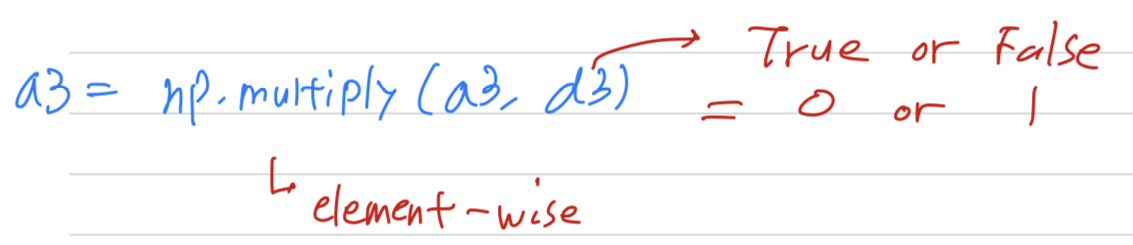
And you gonna set . (element-wise multiplication)
But what this does is for every element of that's equal to zero.
And there was a 20$ chance of each of the elements being zero,
this multiply operation ends up zeroing out, the corresponding element of .
technically will be a boolean array where value is true and false, rather than one and zero.
But the multiply operation works and will interpret the true and false values as one and zero.
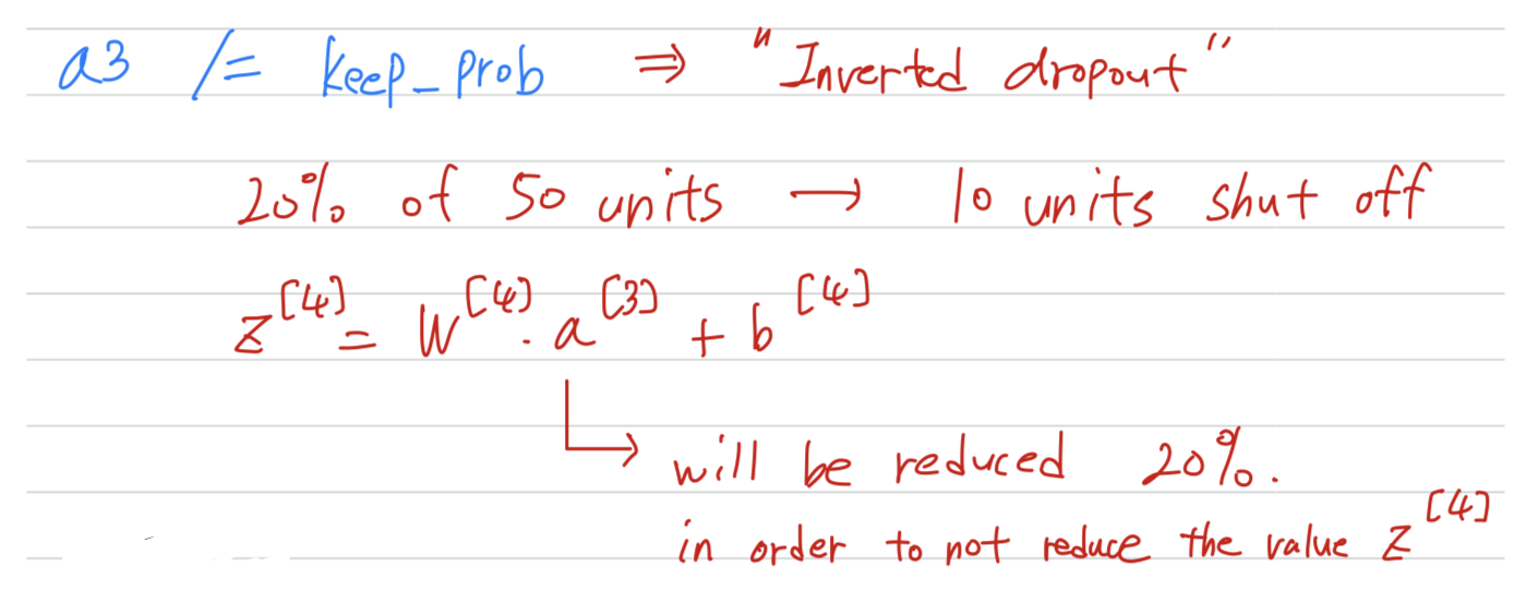
 Then finally, we're going to take and scale it up by dividing by 0.8()
Let's say for the sake of argument that you have 50 units in the 3-hidden layer.
So maybe is (50, 1) dimensional or if you vectorization maybe it's (50, m) dimensional.
So, if you have a 80% chance of keeping them and 20% chance of eliminating them,
this menas that on average, you end up with 10 units shut off or 10 units zeroed out.
And so now, if you look at the value of , .
And so, on expectation, will be reduced by 20%.
By which i mean that 20% of the elements of will be zeored out.
So, in order to not reduce the expected value of ,
what you do is you need to take this, and divide it by 0.8
because this will correct or just a bump that back up by roughly 20% that you need.
So it's not changed the expected value of .
And so this line is what called theinverted dropouttechnique.
And its effect is that no matter whay you say set the to, whether it's 0.8 or 0.9
this inverted dropout techniqe by dividing by the ,
it ensures that the expected value of remains the same.
This makes test time easier because you have less of a scaling problem.
Making predictions at test time
- At test time, you're given some or which you want to make a prediction.
But notice that the test time you're not using dropout explicitly and
you're not tossing coins at random to decide which hidden units to eliminate.
That's because when you are making predictions at the test time,
you don't really want your output to be random.
If you are implementing dropout at test time, that just add noise to your predictions.
Understanding dropout
-
Why does drop-out work as a regulizer?
-
it's as if on every iteration you're working with a smaller neural network.
And so using a smaller neural network seems like it should have a regularizing effect. -
Here's the second intuition which is,
let's look at it from the perspective of a single unit.
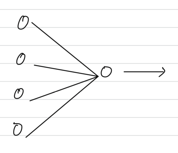 Now with drop-out, the inputs can get randomly eliminated.
Sometimes those two units will get eliminated.
Sometimes a different unit get eliminated.
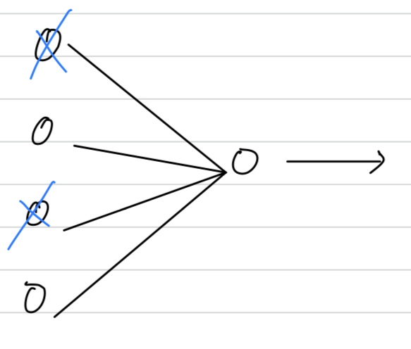 So what this means is that red unit which i'm circling red.
it can't rely on any one feature because anyone feature could go away at random.
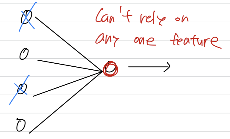
The ways were reluctant to put too much weight on anyone input
because it could go away.
So this unit will be more motivated to spread out this ways and give you a little bit of weight to each of the four inputs to this unit.
And by spreading out the weights
this will tend to have an effect of shrinking the squared norm of the weights.
And so similar to what we saw with L2 regularization,
the effect of implementing dropout is that its strength the ways and similar to L2 regularization,
it helps to prevent overfitting,
but it turns out that dropout can formally be shown to be an adaptive form of L2 regularization,
but the L2 penalty on different ways are different depending on the size of the activation function is being multiplied into that way.
To summarize it is possible to show that dropout has a similar effect to L2 regularization.
Only the L2 reguularization applied to different ways can be a little bit different
and even more adaptive to the scale of different inputs. -
One more detail for when you're implementing dropout, here's a network where you have three input features.
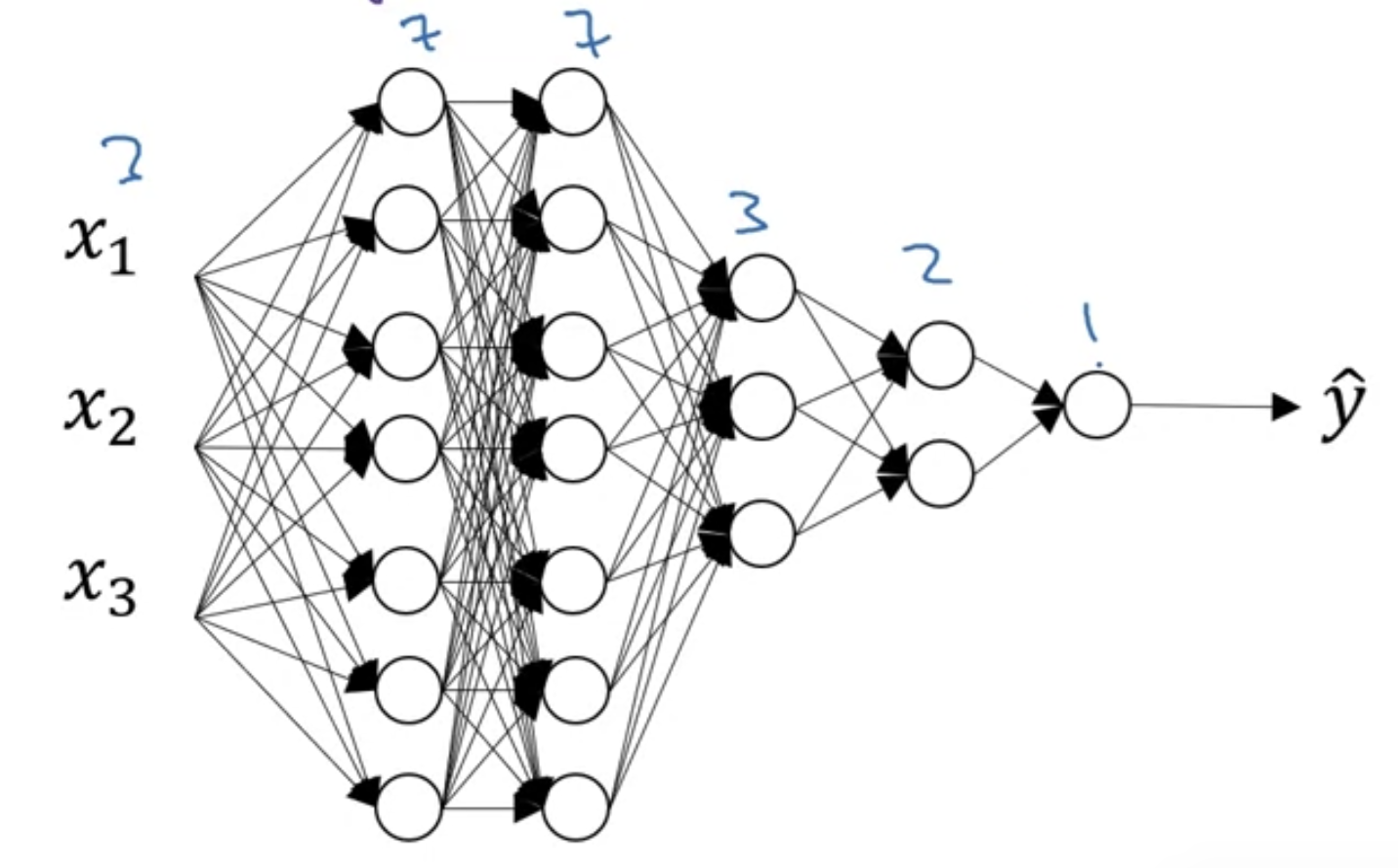 One of the practice we have to choose was the which is a chance of keeping a unit in each layer.
So it is also feasible to vary by layer (layer마다 을 다르게 할 수 있다.)
So to prevent, to reduce overfitting of that matrix, maybe for layer 2,
you might have a that's relatively low, say 0.5,
whereas for different layers where you might worry less about overfitting,
you could have a higher maybe just 0.7.
And then for layers we don't worry about ovefitting at all.
You can have a of 1.0.
Notice that the 1.0 means that you're keeping every unit.
And so you're really not using dropout for that layer.
But for layers where you're more worried about overfitting really the layers with a lot of parameters
you could set to be smaller to applay a more powerful form of dropout.
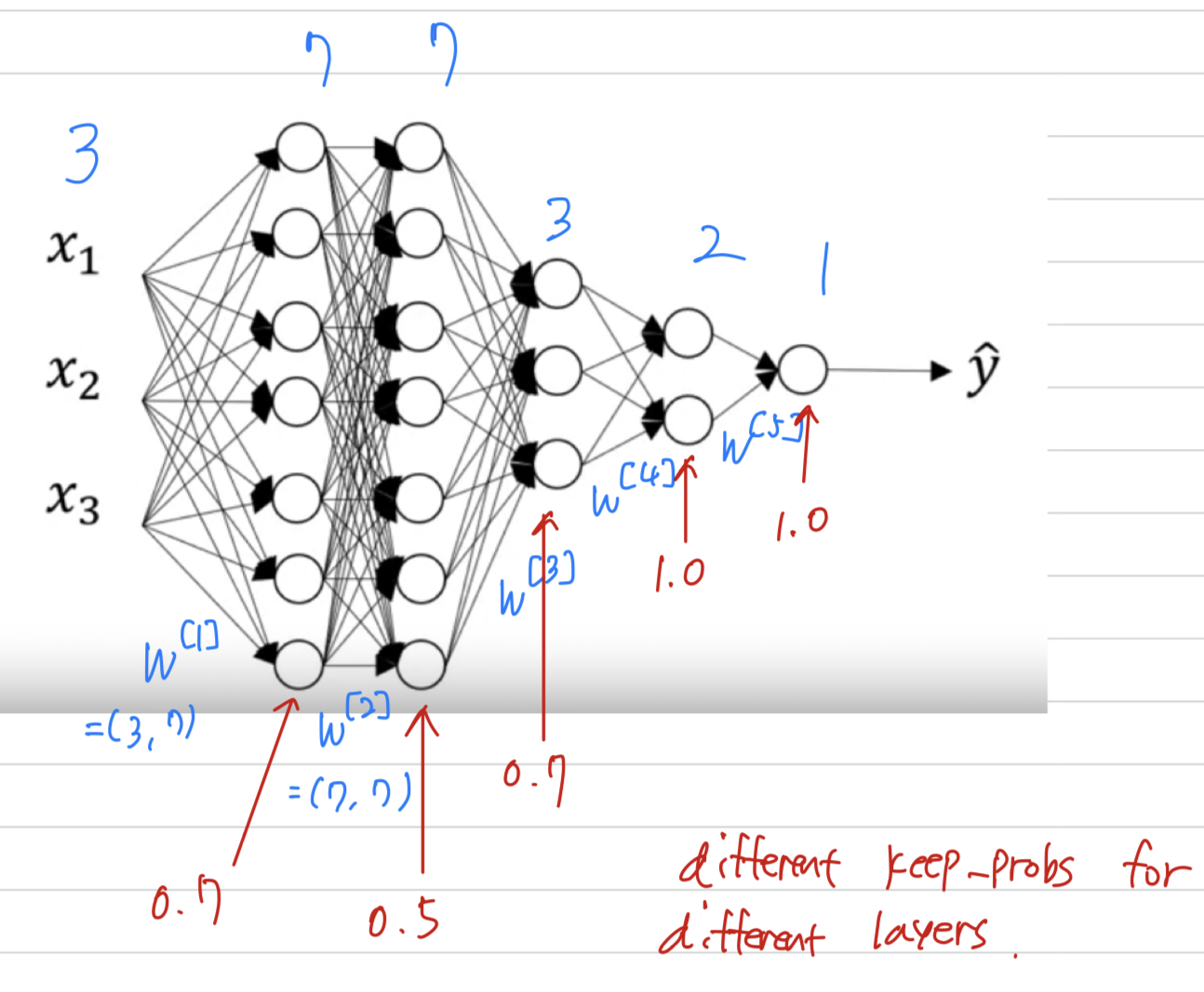
And technically you can also apply dropout to the input layer.
Although in practice, usually don't do that often.
And so of 1.0 is quite common for the input layer.
If you even apply dropout at all will be a number close to 1.
So just to summarize if you're more worried about some layers overfitting than others,
you can set a lower for some layers than others.
The downside is this gives you can more hyper parameters to search for using cross validation.
-
Many of the first successful implementations of dropouts were to computer vision,
so in computer vision, the input sizes so big in putting all these pixels that
you almost never have enough data.
And so dropout is very frequently used by the computer visoin and
there are common vision research is that pretty much always use it almost as a default.But really, the thing to remember is that dropout is a regularization technique,
it helps overfitting.
And so unless my algorithm is overfitting, i wouldn't actually bother to use dropout.
So as you somewhat less often in other application areas, there's just a computer vision,
you usually just don't have enough data so almost always overfitting
, which is why computer vision researchers swear by dropout by the intuition. -
One big downside of dropout is that the cost function is no longer well defined.
On every iteration, you're randomly, calling off a bunch of nodes.
And so if you are double checking the performance of gradient descent
is actually harder to double check that.
You have a well defined cost function .
That is going downhill on every iteration because the cost function that you're optimizing is actually less.
So you use this debugging tool to have a plot a draft like this.
 So what i usually do is turn off dropout and run my code
and make sure that it is monotonically decreasing .
And then turn on dropout and hope that.
I didn't introduce welcome to my code during dropout because you need other ways,
i guess not plotting these figures to make sure that your code is working even with dropout.
So with that there's still a few more regularizationg techniques that were feel knowing.
Let's talk about a few more such techniques in the next.
Other Regularization Methods
- In addition to
L2 regularizationanddropout regularization
there are few other techniques to reducing overfitting in your neural network.
Data augmentation
-
Let's say you fitting a cat classifier.
If you are overfitting getting more training data can help,
but getting more training data can be expensive and sometimes you just can't get more data.
But what you can do is augment your training set by taking image like this.
And for example,(1) flipping it horizontallyand adding that also with your training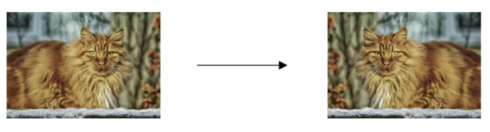 So now instead of just this one example in your training set,
you can add this to your training example.
So by flipping the images horizontally, you could doulbe the size of your training set.
You could do this without needing to pay the expense of going out to take more pictures of cats.
And then other than flipping horizontally,
you can also take(2) random cropsof the image.
So by taking random distortions and translations of the image
you could augment your data set and make additional fake training examples.
 And by synthesizing examples like this what you're really telling your algorithm
is that if something is a cat then flipping it horizontally is still a cat.
Notice i didn't flip it vertically,
because maybe we don't want upside down cats, -
For optical character recognition you can also bring your data set by taking digits and imposing random rotations and distortions to it.
So if you add these things to your training set, these are also still digit force.
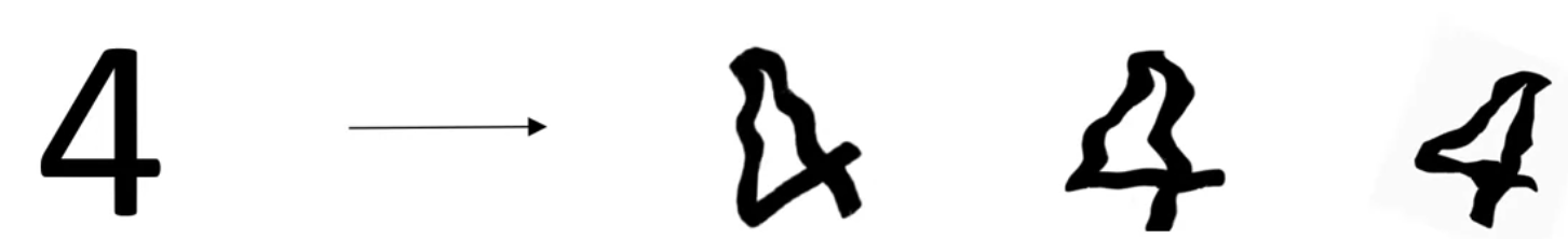
So data augmentation can be used as a regularization technique
Early stopping
-
There's one other technique that is often used called
early stopping. -
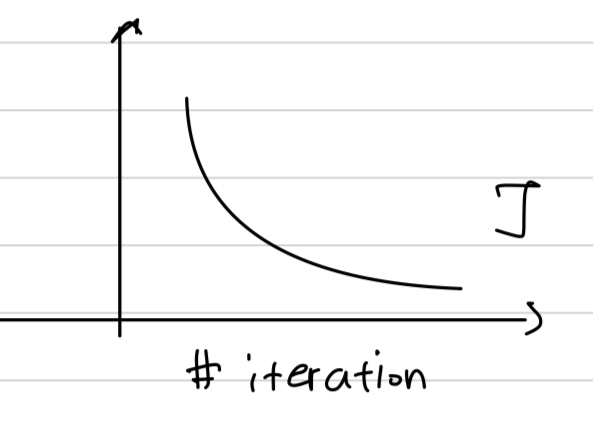
So what you're going to do is as you run gradient descent
you're going to plot either the training error, you'll use 0, 1 classification error on the training set.
Or just plot the cost function optimizing, and that should decrease monotonically like so.
Because as you train, hopefully, you're training error or your cost function should decrease.
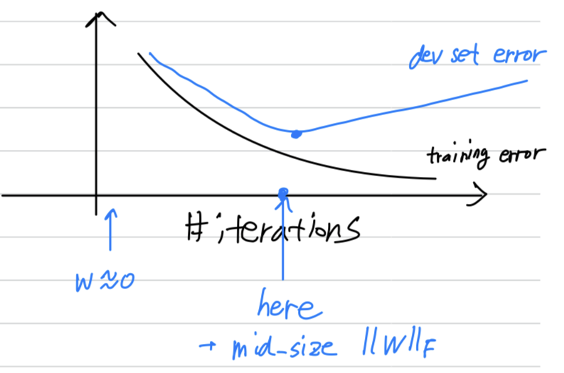
So with early stopping, what you do is you plot this, and youalso plot your dev set error.
And again,
this could be a classification error in a development set
or something like the cost function, like the logistic loss or the log loss of evaluated dev set.
Now what you find is that your dev set error will usually go down for a while,
and then it will increase from there.
So what early stoppig does is, you will say well, it looks like your neural network was doing best around that iteration,
so we just want to stop training on your neural network halfway and take whatever value achieved this dev set error.
So why does this work?
When you've haven't run many iterations for your neural network yet
your parameters will be close to zero
because with random initialization.
You probably initialization to small random values
so before you train for a long time, is still quite small.
And as you iterate, as you train, will get bigger and bigger and bigger until here .
maybe you have a much larger value of the parameters for your neural network.
So what early stopping does is by stopping halfway you have only a mid-size rate .
And so similar to L2 regularization by picking a neural network with similar norm for your parameters ,
hopefully your neural network is overfitting less.
And the termearly stoppingrefers to the fact that
you're just stopping the training of your neural network early.
 But it does have one
 downside.
I think of the machine learning process as comprising several different steps.
One is that you want an algorithm to optimize the cost function J and we have various tools to do that
, such as gradient descent and then we'll talk later about other algorithms like momentum and RMS prop and Adam and so on.
But after optimizing the cost function , you also wanted to not overfit.
And we have some tools to do that such as your regularization, getting more data and so on.
Now in ML, we already have so many hyper-parameters. It surge over.
It's already very complicated to choose among the space of possible algorithms.
The main downside of early stoppinpg is that
this couples these two tasks(optimize cost function J, Not overfit).
So you no longer can work on these two problems independently.
And this principle is sometimes called orthogonalization
(that you want to be able to think about one task at a time.)
(We're going to talk about orthogonalization detail in later video.)
because by stopping gradient descent early you're sort of breaking whatever you're doing to optimize cost function .
And then you also simultaneously trying to not overfit.
So instead of using different tools to solve the two problems, you're using one that that kind of mixes the two.
And this just makes the set of things you could try are more complicated to think about.
Rather than using early stopping,
one alternative is just use L2 regularization
then you can just train the nerual network as long as possible.
I find that this makes the search space of hyper parameters easier to decompose and easier to search over.
But the downside of this though is that you might have to try a lot of values of the regularization parameter .
And so this makes searching over many values of more computationally expensive.
And the advantage of early stopping is that running the gradient descent process just once,
you get to try out values of small , mid-size , and large ,
without needing to try a lot of values of the L2 regularization hyperparameter .
Despite it's disadvantages, many people do use it.
I personally prefer to just use L2 regularization and try different values of .
That's assuming you can afford the computation to do so.
But early stopping does let you get a similar effect
without needing to explicitly try lots of different values of .
Normalizing Inputs
-
When training a neural network , one of the techniques to speed up your training is
if you normalize your inputs. -
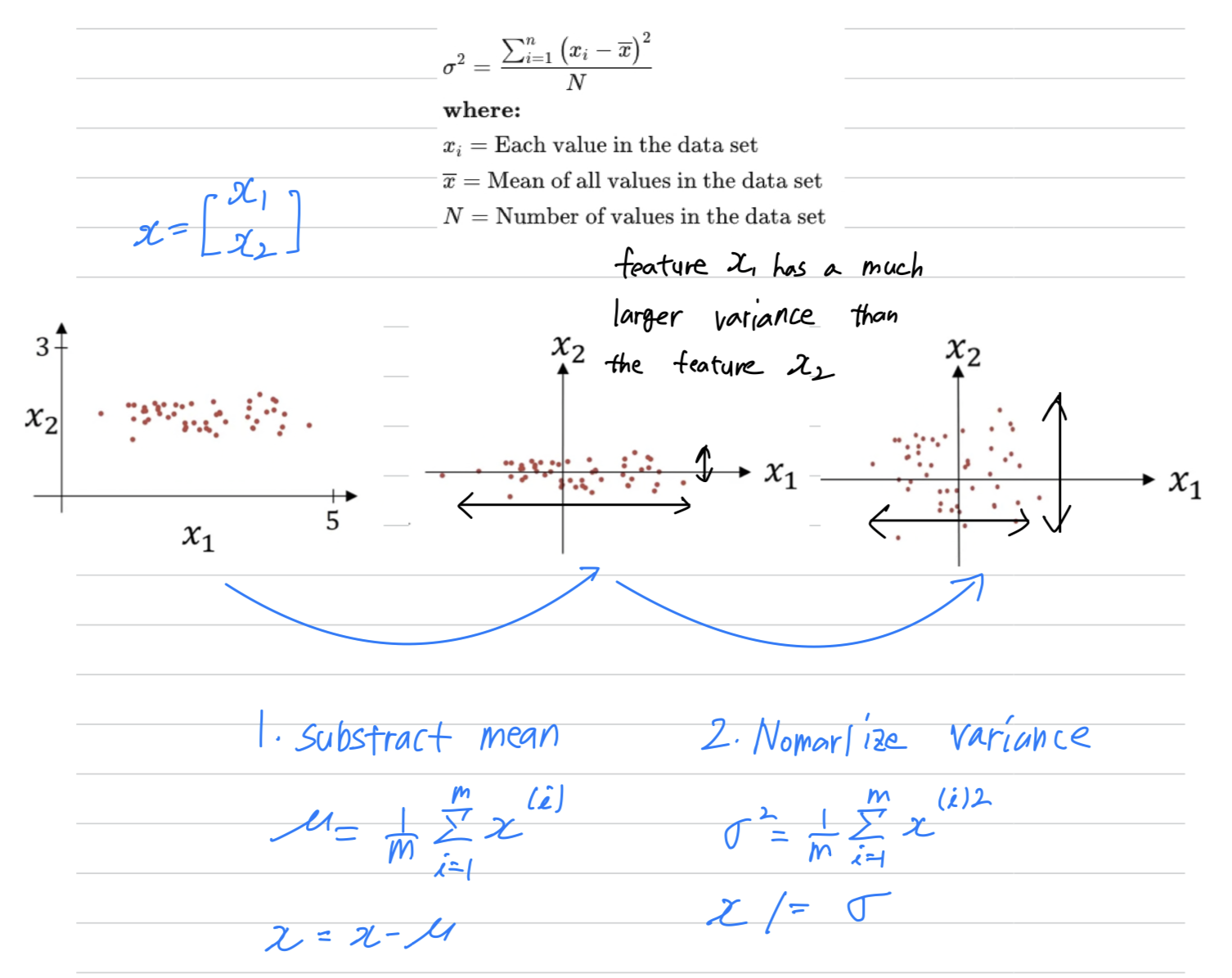
Let's see the training sets with two input features.
Normalizing your inputs corresponds to two steps,
the firstis to substract out or to zero out the mean.
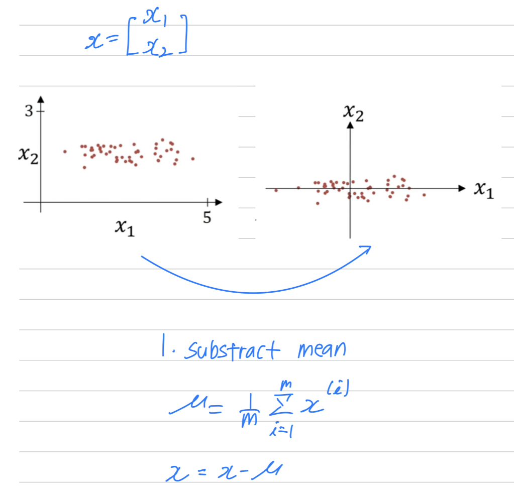 This means that you just move the training set until it has zero mean.
And thenthe secondstep is to normalize the variances.
The feature has a much larger than the feature .
So what we do is set
And so now is a vector with the variances of each of the features.
You take each example and divide it by this vector
You end up with this where now the variance of and are both equal to one.
 One tip if you use this to scale your training data,
then use the same and to normalize your test set.
because you want your data both training and test examples to go through the same transformation
defined by the same and calculated on your training data.
Why normalize inputs?
-
So why do we want to normalize the input features?
-
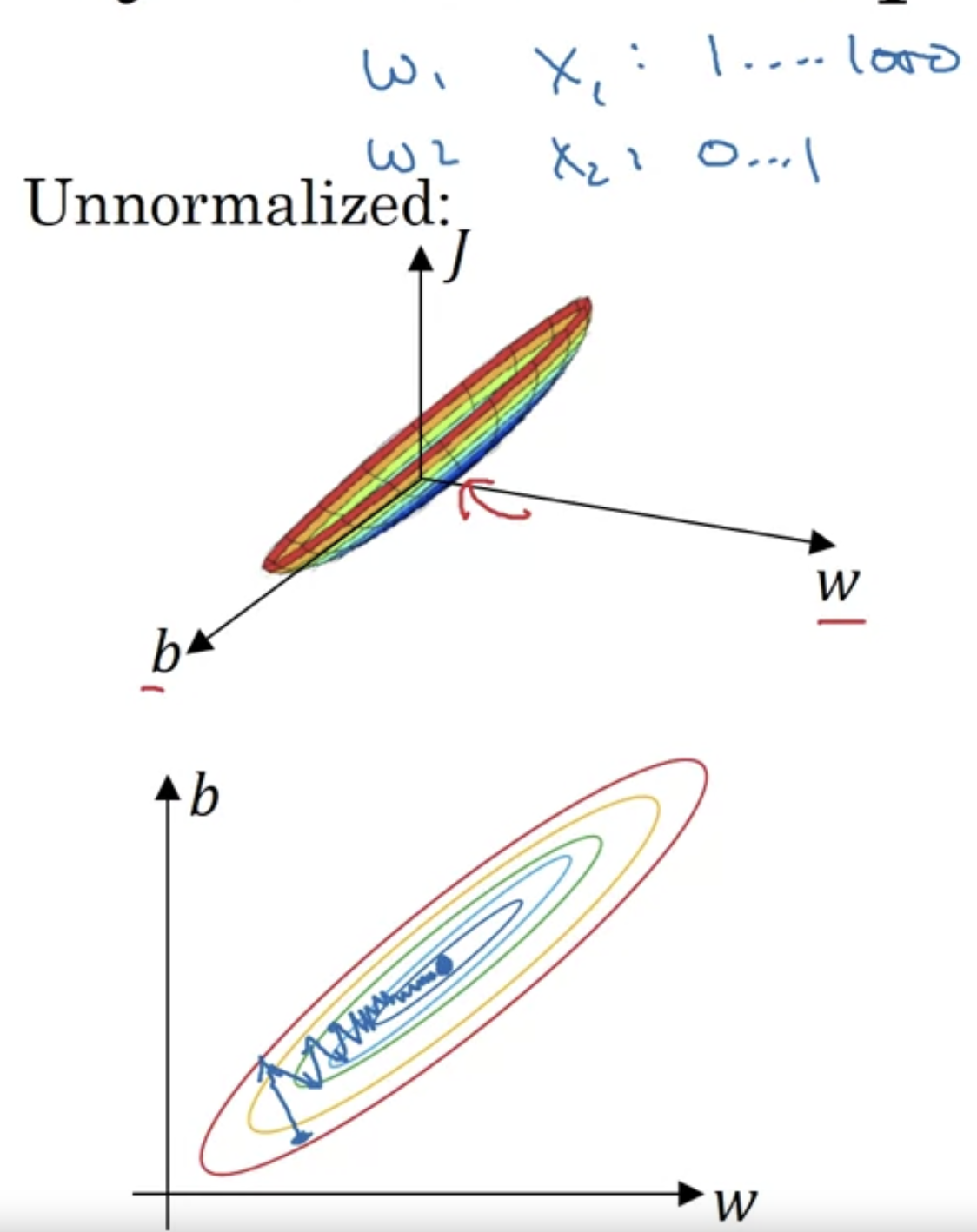
Recall that the cost function is defined as
 It turns out that if you use unnormalized input features,
it's more likely that your cost function will look like this like a very squished out bowl, very elongated cost function where the minimum you're trying to find is maybe over there.
If your features are on very different scales,
say the feature ranges 1~1000, and the feature ranges from 0~1,
then it turns out that the ratio or the range of values for the parameters and
will end up taking on very different values.
And so maybe cost function can be very elongated bowl like that.
 Whereas if you normalize the features,
then your cost function will on average look more symmetric.
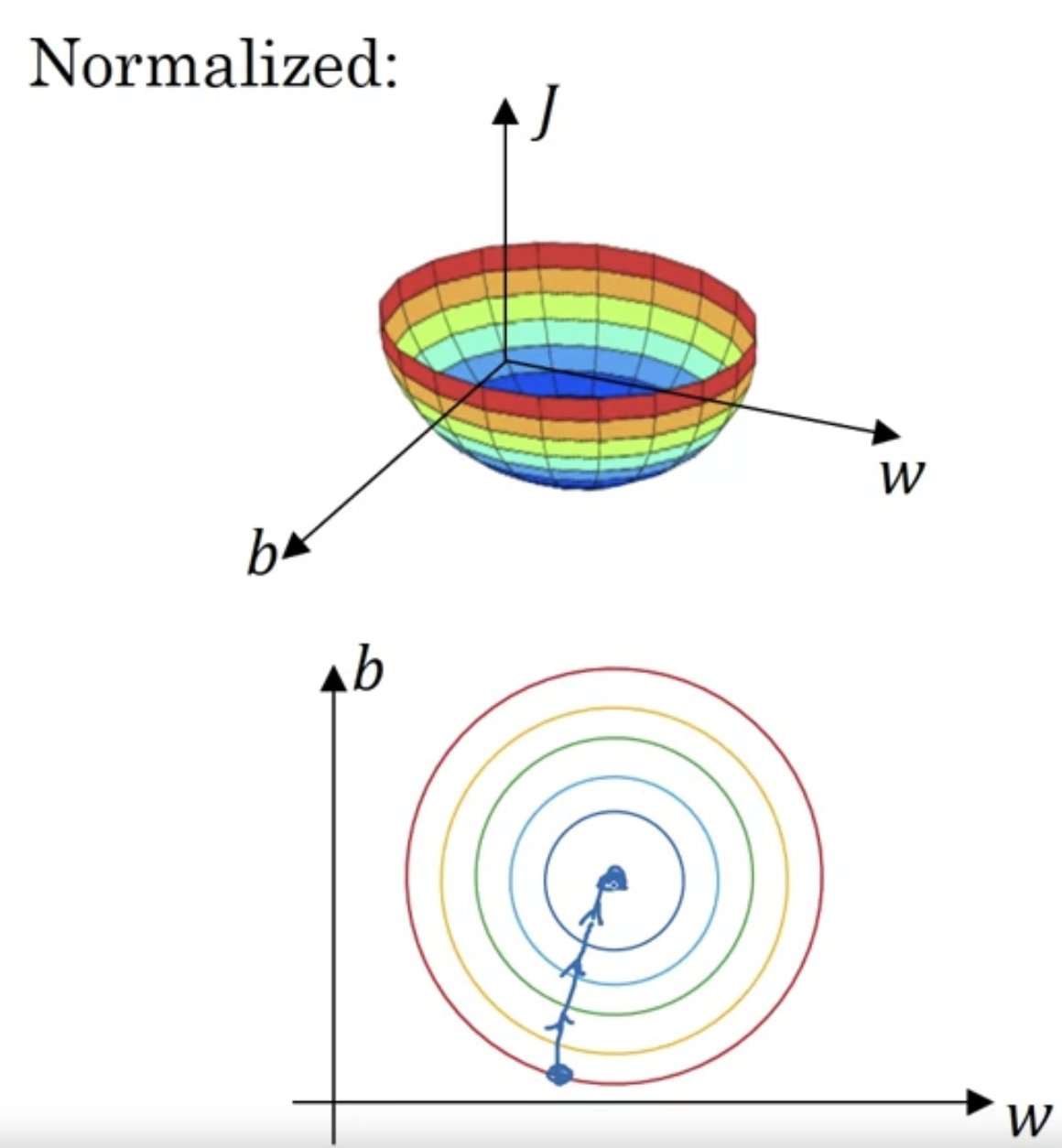 If you are running gradient descent on a cost function like the one on the bottom,
then you might have to use a very small learning rate because if you're here,
the gradient descent might need a lot of steps to oscillate back and forth
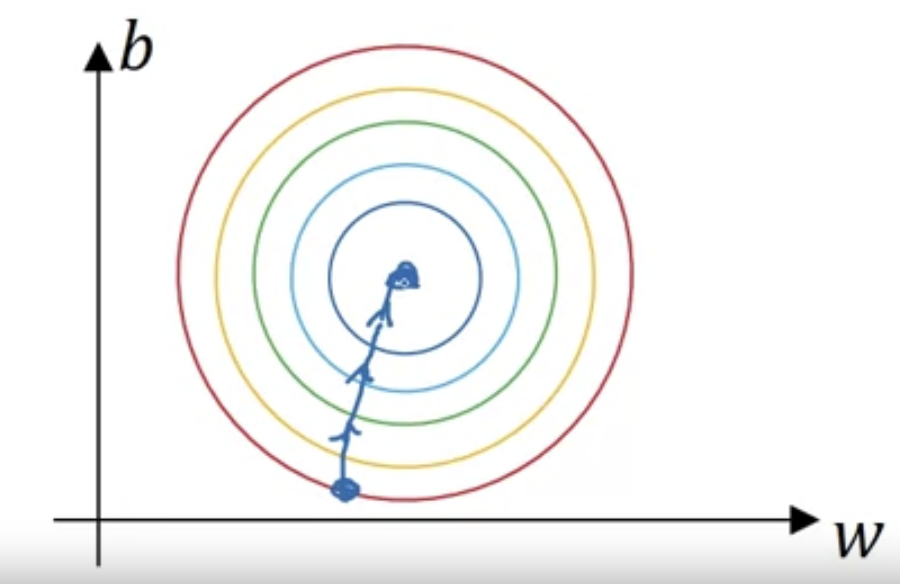
before it finally finds its ways to the minimum.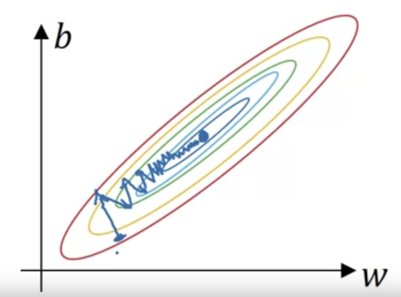 Whereas if you have more spherical contours(구형의 등고선),
then whenever you start , gradient descent can pretty much go straight to the minimum.
You can take much larger steps, where gradient descent need rather than needing to oscillate around like the picture on the top.
So if your input features came from very different scales,
maybe some features are from 0~1, some from 1~1000,
then it's important to normalize your features.
If your features came in on similar scales,
then this step is less important although performing this type of normalization pretty much never does any harm.
Vanishing / Exploding Gradients
-
One of the problems of training neural network, especially very deep neural networks,
isdata vanishingandexploding gradients.
What that means is that when you're training a very deep neural network
your derivatives can sometimes get either very very big or very very small,
maybe even exponentially small and this makes training difficult. -
Unless you're training a very deep neural network like this.
(To save space on the slide, i've drawn it as if you have only 2 hidden units per layer.
but it could be more as well.)
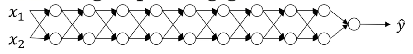 This neural network will have parameter .
For the sake of simplicity, let's say we're using an activation function
so the linear activation function and let's ignore .
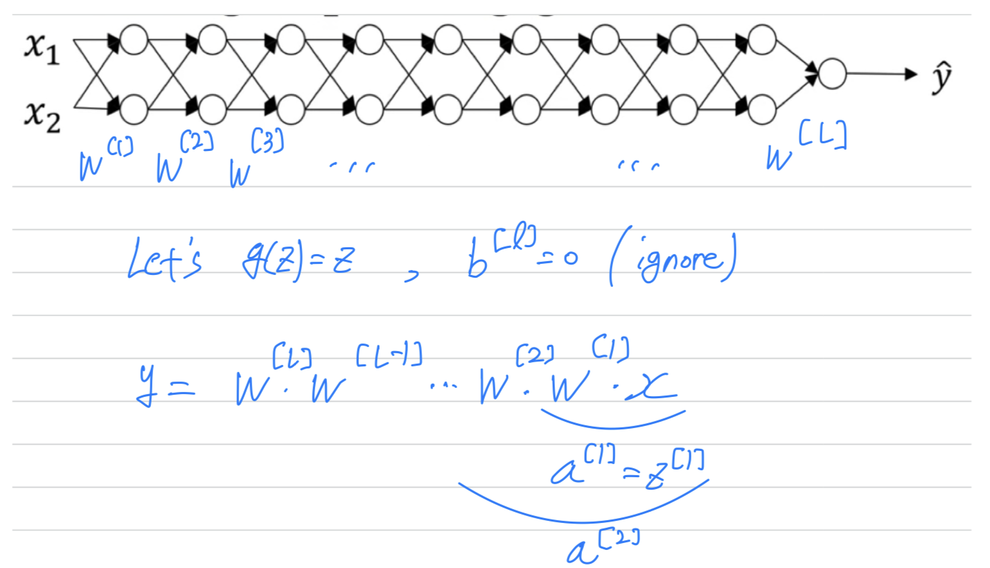 Now, let's say that each of your weight matrices is just a little bit larger than 1 times identity.
So it's 1.5
And so if you have a very deep neural network, the value of will explode.
 Now, conversely, if we replace this with 0.5 so something less than 1.
So in the very deep network, the activations end up decreasing exponentially.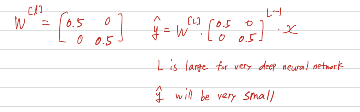
So the intuition i hope you can take away from this
is that at the weight ,
if they're all just a little bit bigger than 1 or just a little bit bigger than the identitiy matrix,
then with a very deep network the activation will explode.
And if is just alittle bit less than identity,
then you have a very deep entwork the activation will decrease exponentially.
Weight initialization for deep networks
-
In the last video we saw how very deep neural networks
can have the problems of vanishing and exploding gradients.
It turns out that a partial solution to this, doesn't solve it entirely but helps a lot,
is better or more careful choice of the rando initialization for your neural network. -
To understand this,
let's start with the example of initializing the weights for a single neuron,
and then we're go on to generalize this to a deep network.
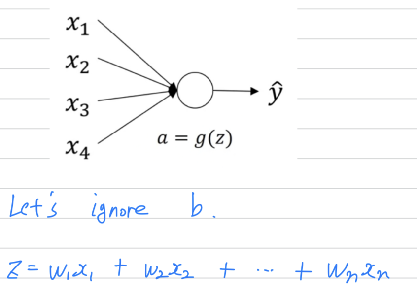 In order to make not blow up and not become too small,
the larger is, the smaller you want .
One reasonalbe thing to do would be to set
where is the number of input features.
So in practice, what you can do is
(개로 나눈 이유 : because that's the number of units that i'm feeding into each of the untis in layer )
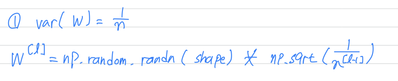 It turns out that if you're using a ReLU activation,
setting in works a little bit better.
It depends on how familiar you are with random variables.
It turns out that something a Gaussian random variable and then multiplying it by a .
So if the input features of activatinos are roughly mean 0 and standard variance 1
then this would cause to also be take on a similar scale.
And this doesn't solve but it definitely helps reduce the vanishing, exploding gradients problem,
because it's trying to set each of the weight matrices ,
so that it's not too much bigger than 1 and too much less than 1
so it doesn't explode or vanish too quickly.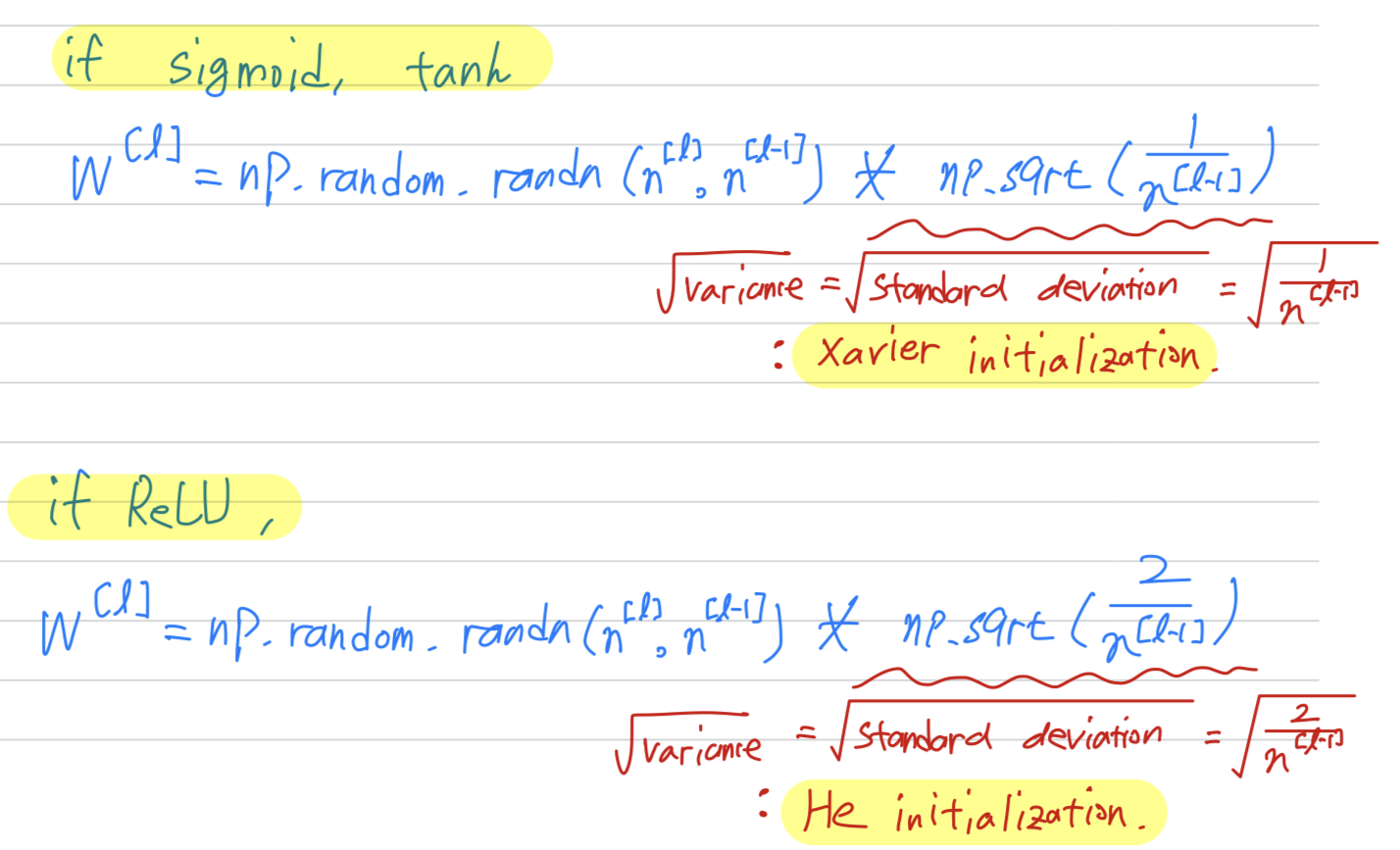
And another version we're taught by Yoshua Bengio and his colleagues,
is to use this formula,
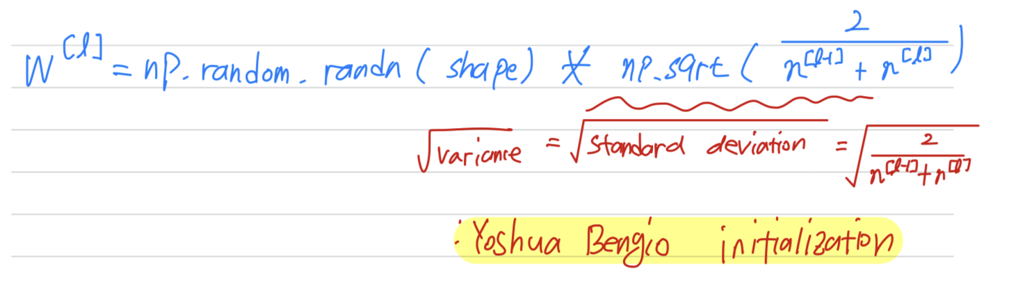 But in practice i think all of these formulas just give you a starting point.
It gives you a default value to use for the variance of the initialization of your weight matrices.
So i hope that gives you some intuition about the problem of vanishing or exploding gradients
as well as choosing a reasonable scailing for how you initialize the weights.
Hopefully that makes your weights not explode too quickly and not decay to zero too quickly,
so you can train a reasonbly deep neural without the weights or gradients exploding or vanishing too much.
Numerical approximation of gradients
-
When you implement back propagation you'll find that there's a test called
gradient checkingthat can really help you make sure that your implementation of backprop is correct. -
So let's take the function
Now instead of just nudging to the right to get ,
and nudge it to the left to get
()
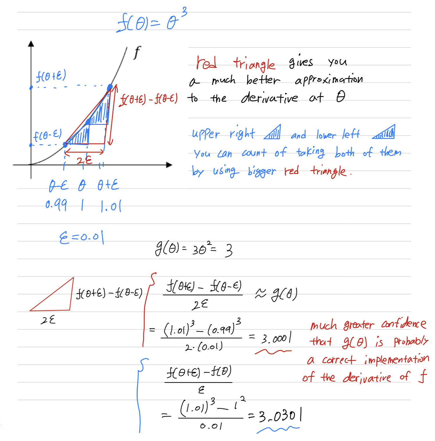 When you use this method for gradient checking and back propagation,
this turns out to run twice as slow as you were to use a one-sided difference.
It turns out that in practice i think it's worth it to use
because it's just much more accurate.This two-sided difference formula is much more accurate.
So that's what we're going to use when we do gradient checking in the next.
Gradient checking
-
Gradient checkingis a technique that's helped me save tons of time,
and helped me find bugs in my implementations of back propagation many times.
Let's see how you could use it to debug or to verify that your implementation and back process correct. -
So to implement
gradient checking,
the first thing you should do is take all your parameters and reshape them into a giant vector data.
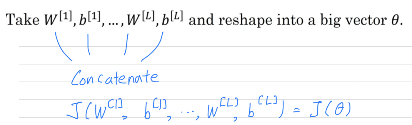 Next, with and ordered the same way,
you can also take and so on, and reshape them into big vector of the same dimension as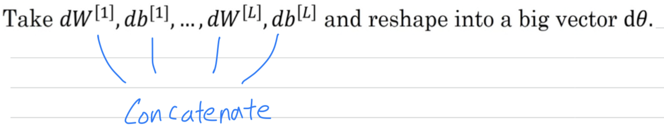 So the question is now,
Is the the gradient or the slop of the cost function ?
-
So here's how you implement gradient checking,
and often abbreviate(줄여 쓰다) gradient checking tograd check.
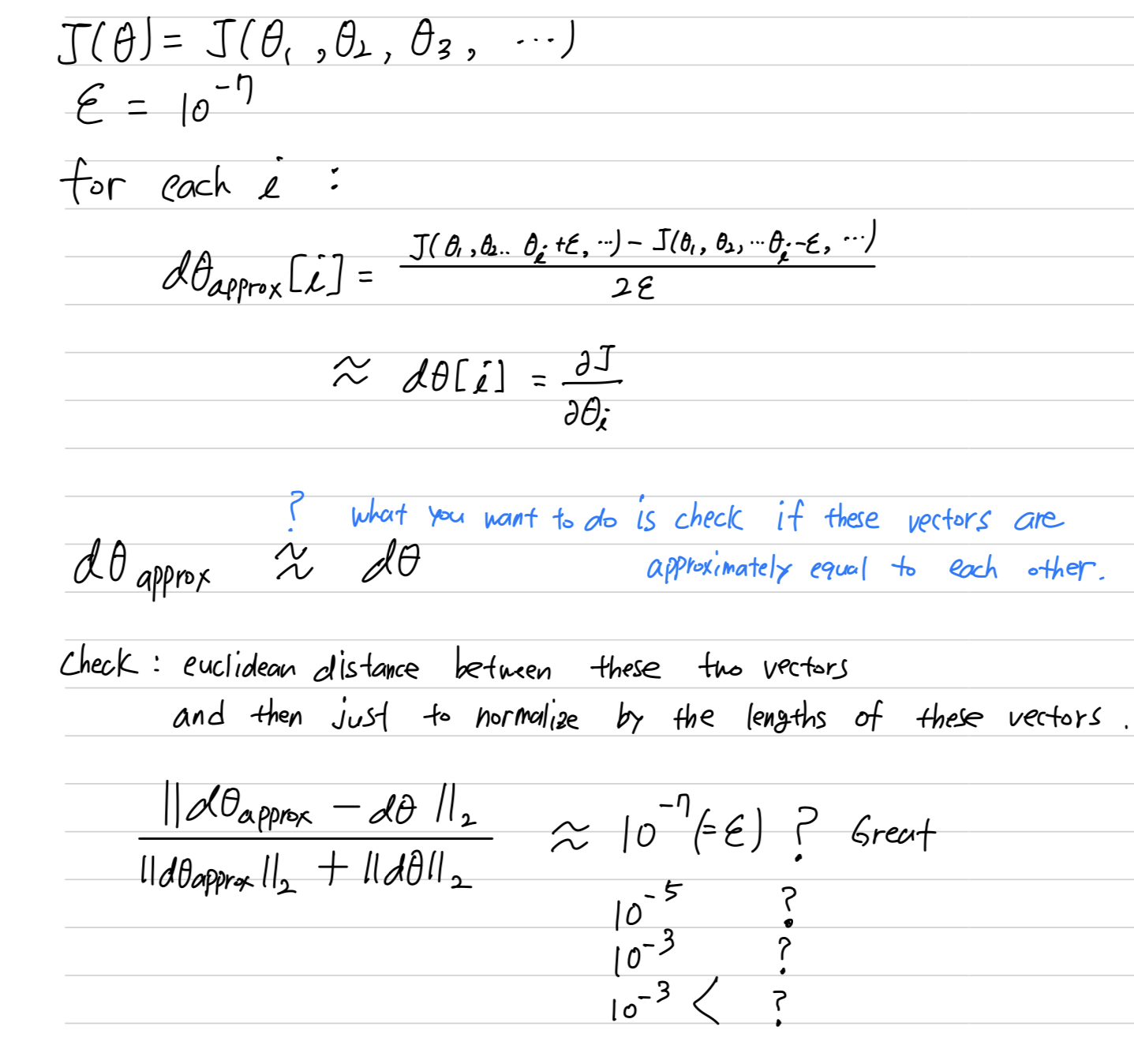
- if you find that this formula gives you a value like , then that's great.
it means that your derivative approximation is very likely correct. - If it's maybe on the range of , i would take a careful look.
Maybe this is okay.
But i might double-check the components of this vector,
and make sure that none of the components are too large.
And if some of the components of this difference are very large,
then maybe you have a bug somewhere. - If it's maybe on the range of , then i would worry that there's a bug somewhere.
- If any bigger than , then i would be quite concerned.
I would be seriously worried that there might be a bug.
And you should look at the individual components of data
to see if there's a speicific value of for is very different from .
- if you find that this formula gives you a value like , then that's great.
Gradient Checking implementation notes
- In this video, i want to share with you some practical tips or some notes
on how to actually go about implementing this for your neural network.
-
Don't use
grad checkin training, only to debug.
So what i mean is that, computing a for all the values of ,
this is a very slow computation.
So to implement gradient descent,
you'd use backprop to compute just use backprop to compute the derivative.
And it's only when you're debugging that you would compute this
to make sure it's close to .
But once you've done that, then you would turn off the grad check,
and don't run this during every iteration of gradient descent. -
if an algorithms fails grad check, look at the componenets to try to identify bug.
So what i mean is that if is very far from ,
what i would do is look at the different values of to see
which are the values of that are really very different than the .
So for example, if you find that the values of or , they're very far off,
all correspond for some layers, but the components for are quite close.
Remember, different components of correspond to different components of and .
When you find this is the case, then maybe you find that the bug is in
how you're computing , the derivative with respect to parameters .
This doesn't always let you identify the bug right away,
but sometimes it helps you give you some guesses about where to track down the bug. -
When doing grad check, remember your regularization term if you're using regularization.
So if your cost function .
And you should have that is gradient of respect to including this regularization term.
So just remember to include the term. -
Grad check doesn't work with dropout.
because in every iteration, dropout is randomly eliminating different subsets of the hidden units.
There isn't an easy to compute cost function that dropout is doing gradient descent on.
It turns out that dropout can be viewed as optimizing some cost function ,
but it's cost function defined by summing over all exponentially large subsets of nodes
they could eliminate in any iteration.
So the cost function is very difficult to compute,
and you're just sampling the cost function every time you eliminate different random subsets in those we use dropout.
So if you want, you can set and dropout to be equal to 1.0.
And then turn on dropout and hope that my implementation of dropout was correct. -
Finally, this is a subtlety.
It is not impossible, rarely happens, but is's not impossible that
your implementation of gradient descent is correct when and are close to 0,
so at random initializatoin.
But that as you run gradient descent and and become bigger,
maybe your implementation of backprop is correct only when and is close to 0,
but it gets more inaccurate when and become large.
One thing you could do is run grad check at random initialization
and then train the network for a while so that and have sometime to wander away from 0,
from your small random initial values.
Quiz
모르겠는 부분
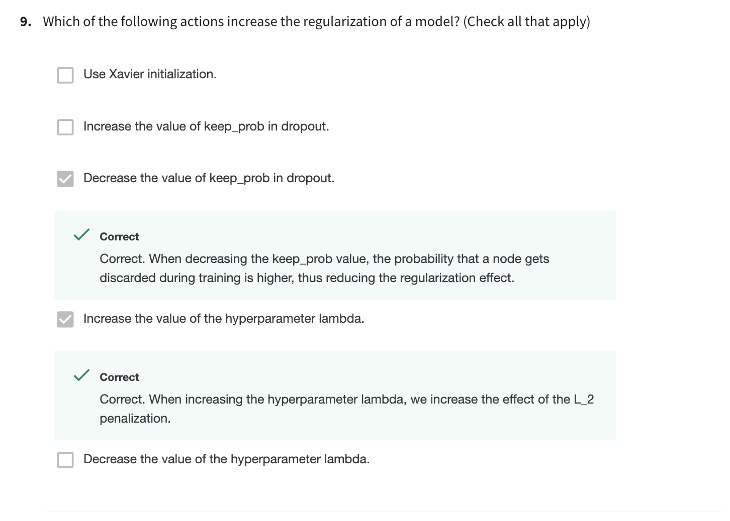
- If you use L1 regularization, then will end up being sparse.
- dropout을 적용한다면, 왜 cost function J가 잘 정의되지 않는가?
- weight initilization에서 왜 weight의 variance를 = 로 initialization하는가?
Seminar - discussion
-
인공지능 > 머신러닝 > 딥러닝인데, 머신러닝과 딥러닝은 뭐가 다른가?
-
머신러닝은 machine이 data로 부터 학습을 한다.
data가 많이 필요하지 않은 작은 model에 사용하는 것이 대부분이다.
preivous era : 보통 적은 layer ➡️ data가 많이 필요하지 않음. -
딥러닝은 model이 깊어지고, data의 dimension이 커짐. (화질, 크기, 단순하지 않은 온갖 종류의 물체)
문제가 어려워지고, data도 커지고, 처리하기 위한 model 학습이 어려워짐.
train한다는 말은 == parameter를 update한다는 말이다.
parameter update에 사용되는 data는 train set밖에 없다.
어려운 문제를 풀기 위해 prarmeter update하는 train data가 늘어날 수밖에 없다.
그래서 현대에는 dev, test set의 비율이 줄어드는 것이다.
또한 대부분 dev set과 test set을 하나로 본다.
train 도중에 dev set을 통해 model을 test하는 것이기 때문에 dev set은 parameter update에 간접적으로 작용한다.
development set(dev set)은 보통 validation set(val set)이라고 한다.
-
-
val set과 test set의 distribution이 같아야 좋다.
- dev set으로 train시키는데, 그것에 맞춰져있는 model이
다른 test set distribution에 적용한다면 당연히 accuracy가 달라진다.
그래서 dev set과 test set의 distribution은 같아야 한다. - 머신러닝의 목적은 generalization이다 == train에서 잘 된 것이 test에서도 잘 돼야 한다.
train에서만 잘 되는 것은 generalization이 안되는 것이다.
소수의 set(train set)에서만 잘되는 것임.
하지만 현실적으로 distribution이 조금은 다를 수 밖에 없다..
- dev set으로 train시키는데, 그것에 맞춰져있는 model이
-
High bias, High variance는 딥러닝에서 잘 사용하는 용어가 아니다.
보통 Underfitting, Overfitting이라고 한다. -
Overfitting을 극복하는 것은 data가 많은 것이 가장 좋다.
하지만 현실적으로 어렵기 때문에 regularization 등을 하는 것이다. -
regularization은 Overfitting을 줄이기 위한 포괄적인 방법이다.
regularization에는 구체적으로 L1, L2, dropout, data augmentation 등이 있다. -
L2 regularization :
- weight를 작게 만들어서 sigmoid나 tanh의 linear(x축이 0에 가까움)한 부분의 값을 갖도록 한다 ➡️ NN을 멍청하게 만든다 ➡️ Overfitting을 완화
- 큰 값을 줄이는 역할도 있다.
-
iteration : dataset의 일부분이 forward & backward 과정 1번
epoch : 전체 dataset을 모두 forward & backward 과정 1번- data의 일부분 X 5 = 전체 data set 이라면,
5 iterations = 1 epoch
매 epoch마다 Loss를 monitoring하는 것은 오래 걸리지 않아서 항상 하는 것이 좋다.
- data의 일부분 X 5 = 전체 data set 이라면,
-
대부분 Early stopping point까지 돌려보다가 training을 종료한다.
처음 epoch을 300으로 설정하고 Early stopping의 epoch이 100이었다면,
두번째 학습에서는 120까지만 돌려본다. -
학습 중에 값은 커질수도 있고, 작아질 수도 있다.
이기 때문에 dW에 따라 커질 수도, 작아질 수도 있. -
이미지의 밝기를 조절하는 것, blurring하는 것도 data augmentation의 일종이다.
-
cat image에서는 $x_1, x_2,... $ feature들의 분포 차이가 크지 않다.
image는 0~255 사이의 값을 갖기 때문에 /255 연산을 해줘서 0~1로 변환해준다.
그래서 보통 image는 /255로 input normalization을 한다.
다른 dataset 같은 경우(분포가 서로 많이 다른 경우 = feature 간 scale이 다른 경우)는
normal distribution(평균 0, 분산 1)으로 만들어준다. -
feature 간의 scale이 다르다면(unnormalized), backward과정에서 이기 때문에
그래프는 길쭉, 찌그러진 이상한 function이 된다.
그래서 gradient descent가 오래 걸린다.
즉, unnormalized feature 로 train한다면, overshooting(loss의 최저점을 지나치는 현상)이 일어나서 학습이 오래걸린다.
normalized feature 로 train한다면, overshooting 현상이 잘 안생겨서 학습이 보다 빠르다. -
He initialization에서 분산을 2배 해주는 이유 :
ReLU를 통과하는 순간 절반이 날아가기 때문에,
분산이 반으로 줄어든다. 따라서 분산에 2를 곱해준다. -
depth가 작으면, Gradient vanishing이 생기지 않는다.
depth가 작은 model의 weight initialization에서 x0.01을 하지 않아도 학습을 잘 되었을 것이다.
