이전의 코드를 파이토치 버전으로 작성했다.
from torchvision.datasets import FashionMNIST
from sklearn.model_selection import train_test_split
import torch.nn as nn
from torchinfo import summary
import torch
import torch.optim as optim
import matplotlib.pyplot as plt

# 데이터 불러오기
fm_train = FashionMNIST(root='.', train=True, download=True)
fm_test = FashionMNIST(root='.', train=False, download=True)

# 데이터 사이즈 확인
print(fm_train.data.shape, fm_test.data.shape)
# torch.Size([60000, 28, 28]) torch.Size([10000, 28, 28])

# input, taget 분리
train_input = fm_train.data
train_target = fm_train.targets

# 정규화
train_scaled = train_input / 255.0


# 데이터 분리
train_scaled, val_scaled, train_target, val_target = train_test_split(train_scaled, train_target, test_size=0.2, random_state=42)

# 데이터 크기 확인
print(train_scaled.shape, val_scaled.shape)
# torch.Size([48000, 28, 28]) torch.Size([12000, 28, 28])

model = nn.Sequential(
    nn.Flatten(), # 28*28 데이터를 1차원(784개)으로 평탄화
    nn.Linear(784, 100),  # 784개의 테이터를 100개로
    nn.ReLU(),    # 활성화 함수로 ReLU 사용
    nn.Linear(100,10) # 100개의 데이터를 10개로
    # 파이토치에서는 softmax 생략(이후 손실 함수를 사용할 때 softmax가 포함되어있음)
)

# keras의 summary
print(summary(
    model,
    input_size=(32, 28, 28) # 배치 사이즈 32, 28*28 데이터
))

==========================================================================================
Layer (type:depth-idx)                   Output Shape              Param #
==========================================================================================
Sequential                               [32, 10]                  --
├─Flatten: 1-1                           [32, 784]                 --
├─Linear: 1-2                            [32, 100]                 78,500
├─ReLU: 1-3                              [32, 100]                 --
├─Linear: 1-4                            [32, 10]                  1,010
==========================================================================================
Total params: 79,510
Trainable params: 79,510
Non-trainable params: 0
Total mult-adds (M): 2.54
==========================================================================================
Input size (MB): 0.10
Forward/backward pass size (MB): 0.03
Params size (MB): 0.32
Estimated Total Size (MB): 0.45
==========================================================================================

# GPU있는 경우 GPU 사용
device = torch.device("cuda" if torch.cuda.is_available() else "cpu")
model.to(device)

# 손실 함수 CrossEntropyLoss 사용
# 파이토치의 crossentropyLoss에는 softmax가 포함되어있다.
criterion = nn.CrossEntropyLoss()

"""
만약 다중 분류 손실 함수로 NLLLoss를 사용하는 경우에는 모델의 마지막에 LogSoftmax 층을 추가해야 한다.

model = nn.Sequential(
    nn.Flatten(),
    nn.Linear(784, 100),
    nn.ReLU(),
    nn.Linear(100,10),
    nn.LogSoftmax(dim=1)
    # dim = 1: 각 행(샘플) 안에서 클래스별로 확률 계산
    # dim = 0: 각 열(클래스) 방향으로 확률 계산

)

criterion = nn.NLLLoss()
""";

# 옵티마이저 Adam 사용
optimizer = optim.Adam(model.parameters())
# model.parameters: 훈련 가능한 모든 모델 파라미터를 전달함

EPOCHS = 20
BATCH_SIZE = len(train_scaled) // 32

acc_lst = []
loss_lst = []
for epoch in range(EPOCHS):
    model.train()   # 모델 훈련 모드로 변경
    train_loss = 0  # 훈련 손실 값
    train_acc = 0   # 훈련 정확도 값

    for i in range(BATCH_SIZE):
        # 배치 사이즈 만큼 데이터 추출
        inputs = train_scaled[i*32:(i+1)*32].to(device)
        targets = train_target[i*32:(i+1)*32].to(device)

        # 옵티마이저 기울기 초기화
        optimizer.zero_grad()
        # 출력 얻음
        outputs = model(inputs)

        # 출력값과 타깃을 비교하여 loss 계산
        loss = criterion(outputs, targets)

        # 파라미터에 대한 기울기를 계산
        loss.backward()
        # 계산된 기울기를 기반으로 모델 파라미터 업데이트
        optimizer.step()

        train_loss += loss.item()

        preds = outputs.argmax(dim=1)  # 각 샘플에서 최대값 인덱스
        train_acc += (preds == targets).sum().item()

    # acc, loss 계산하기
    avg_loss = round(train_loss/BATCH_SIZE, 4)
    avg_acc = round(train_acc/len(train_scaled), 4)

    loss_lst.append(avg_loss)
    acc_lst.append(avg_acc)

    print(f"epoch: {epoch+1}, acc: {avg_acc}, loss: {avg_loss}")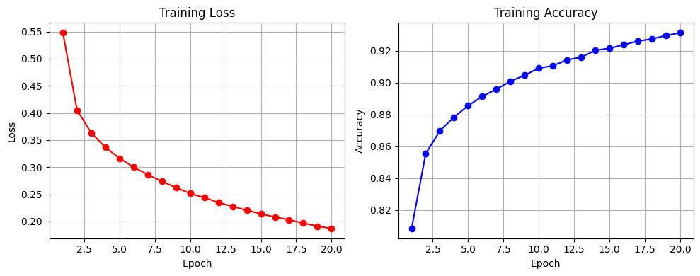

코딩 공부하는 사람