1. 파이토치로 구현하기

---

import torch
import torch.nn as nn
import torch.nn.functional as F
import torch.optim as optim

torch.manual_seed(1)

# 훈련 데이터
x1_train = torch.FloatTensor([[73], [93], [89], [96], [73]])
x2_train = torch.FloatTensor([[80], [88], [91], [98], [66]])
x3_train = torch.FloatTensor([[75], [93], [90], [100], [70]])
y_train = torch.FloatTensor([[152], [185], [180], [196], [142]])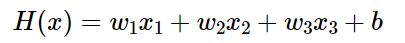

기본세팅 및 훈련데이터를 설정할 것인데, 단순선형회귀와 다르게 x변수의 개수가 3개이므로 x_train도 3개를 설정

# 가중치 w와 편향 b 초기화
w1 = torch.zeros(1, requires_grad=True)
w2 = torch.zeros(1, requires_grad=True)
w3 = torch.zeros(1, requires_grad=True)
b = torch.zeros(1, requires_grad=True)

가중치와 편향도 0으로 초기화해주었다.

# optimizer 설정
optimizer = optim.SGD([w1, w2, w3, b], lr=1e-5)

nb_epochs = 1000
for epoch in range(nb_epochs + 1):

    # H(x) 계산
    hypothesis = x1_train * w1 + x2_train * w2 + x3_train * w3 + b

    # cost 계산
    cost = torch.mean((hypothesis - y_train) ** 2)

    # cost로 H(x) 개선
    optimizer.zero_grad()
    cost.backward()
    optimizer.step()

    # 100번마다 로그 출력
    if epoch % 100 == 0:
        print('Epoch {:4d}/{} w1: {:.3f} w2: {:.3f} w3: {:.3f} b: {:.3f} Cost: {:.6f}'.format(
            epoch, nb_epochs, w1.item(), w2.item(), w3.item(), b.item(), cost.item()
        ))

Epoch    0/1000 w1: 0.294 w2: 0.294 w3: 0.297 b: 0.003 Cost: 29661.800781
Epoch  100/1000 w1: 0.674 w2: 0.661 w3: 0.676 b: 0.008 Cost: 1.563628
Epoch  200/1000 w1: 0.679 w2: 0.655 w3: 0.677 b: 0.008 Cost: 1.497595
Epoch  300/1000 w1: 0.684 w2: 0.649 w3: 0.677 b: 0.008 Cost: 1.435044
Epoch  400/1000 w1: 0.689 w2: 0.643 w3: 0.678 b: 0.008 Cost: 1.375726
Epoch  500/1000 w1: 0.694 w2: 0.638 w3: 0.678 b: 0.009 Cost: 1.319507
Epoch  600/1000 w1: 0.699 w2: 0.633 w3: 0.679 b: 0.009 Cost: 1.266222
Epoch  700/1000 w1: 0.704 w2: 0.627 w3: 0.679 b: 0.009 Cost: 1.215703
Epoch  800/1000 w1: 0.709 w2: 0.622 w3: 0.679 b: 0.009 Cost: 1.167810
Epoch  900/1000 w1: 0.713 w2: 0.617 w3: 0.680 b: 0.009 Cost: 1.122429
Epoch 1000/1000 w1: 0.718 w2: 0.613 w3: 0.680 b: 0.009 Cost: 1.079390

이제 optimizer, model, cost function을 설정해주고 epoch을 1000으로 준 후 훈련시키면 위와 같은 결과가 나온다.

2. 벡터와 행렬 연산으로 바꾸기

---

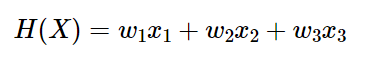
위에서 사용했던 모델 식은 아래와 같이 두 벡터의 Dot product로 표현 가능하다.

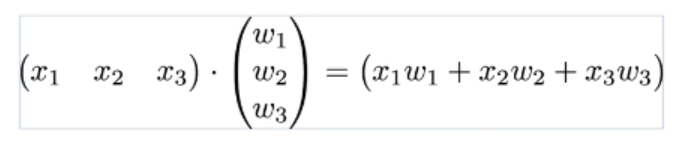
두 벡터를 각각 X 와 W로 표현한다면 모델은 H(X) = XW 로 나타낼 수 있다.

입력 변수 x의 개수가 3개였음에도 이제는 X와 W라는 2개의 변수로 표현된 것을 볼 수 있다.

3. 행렬 연산을 고려하여 파이토치로 구현

---

x_train  =  torch.FloatTensor([[73,  80,  75], 
                               [93,  88,  93], 
                               [89,  91,  80], 
                               [96,  98,  100],   
                               [73,  66,  70]])  
y_train  =  torch.FloatTensor([[152],  [185],  [180],  [196],  [142]])

행렬 연산을 고려하여 모델을 구현할 것이기 때문에 x_train, y_train 또한 행렬로 선언해야한다.

print(x_train.shape)
print(y_train.shape)

torch.Size([5, 3])
torch.Size([5, 1])

x_train과 y_train의 크기가 각각 (5x3), (5x1)로 나왔음을 알 수 있다.

# 가중치와 편향 선언
W = torch.zeros((3, 1), requires_grad=True)
b = torch.zeros(1, requires_grad=True)

다음 과정으로 가중치와 편향을 선언했는데 여기서 주목할 점은 W의 크기가 (3x1)이라는 점이다.

X의 크기가 (5x3)이고 Y의 크기가(5x1)이므로, W는 (3x1)이어야 Dot product가 정의된다.

hypothesis = x_train.matmul(W) + b

가설(모델)을 행렬곱으로 나타내면 위와 같다.

4. 전체코드

---

import torch
import torch.nn as nn
import torch.nn.functional as F
import torch.optim as optim

torch.manual_seed(1)

# 데이터
x_train  =  torch.FloatTensor([[73,  80,  75],
                               [93,  88,  93],
                               [89,  91,  80],
                               [96,  98,  100],
                               [73,  66,  70]])
y_train  =  torch.FloatTensor([[152],  [185],  [180],  [196],  [142]])

# 모델 초기화
W = torch.zeros((3, 1), requires_grad=True)
b = torch.zeros(1, requires_grad=True)

# optimizer 설정
optimizer = optim.SGD([W,b], lr=1e-5)

nb_epochs = 20
for epoch in range(nb_epochs + 1):

    # H(x) 계산, b는 브로딩캐스팅되어 각 샘플에 더해짐
    hypothesis = x_train.matmul(W) + b

    # cost 계산
    cost = torch.mean((y_train - hypothesis) ** 2)

    # 최적화
    optimizer.zero_grad()
    cost.backward()
    optimizer.step()

    print('Epoch {:4d}/{} hypothesis: {} Cost: {:.6f}'.format(
        epoch, nb_epochs, hypothesis.squeeze().detach(), cost.item()
    ))

Epoch    0/20 hypothesis: tensor([0., 0., 0., 0., 0.]) Cost: 29661.800781
Epoch    1/20 hypothesis: tensor([66.7178, 80.1701, 76.1025, 86.0194, 61.1565]) Cost: 9537.694336
Epoch    2/20 hypothesis: tensor([104.5421, 125.6208, 119.2478, 134.7862,  95.8280]) Cost: 3069.590088
Epoch    3/20 hypothesis: tensor([125.9858, 151.3882, 143.7087, 162.4333, 115.4844]) Cost: 990.670288
Epoch    4/20 hypothesis: tensor([138.1429, 165.9963, 157.5768, 178.1071, 126.6283]) Cost: 322.481873
Epoch    5/20 hypothesis: tensor([145.0350, 174.2780, 165.4395, 186.9928, 132.9461]) Cost: 107.717064
Epoch    6/20 hypothesis: tensor([148.9423, 178.9730, 169.8976, 192.0301, 136.5279]) Cost: 38.687496
Epoch    7/20 hypothesis: tensor([151.1574, 181.6346, 172.4254, 194.8856, 138.5585]) Cost: 16.499043
Epoch    8/20 hypothesis: tensor([152.4131, 183.1435, 173.8590, 196.5043, 139.7097]) Cost: 9.365656
Epoch    9/20 hypothesis: tensor([153.1250, 183.9988, 174.6723, 197.4217, 140.3625]) Cost: 7.071114
Epoch   10/20 hypothesis: tensor([153.5285, 184.4835, 175.1338, 197.9415, 140.7325]) Cost: 6.331847
Epoch   11/20 hypothesis: tensor([153.7572, 184.7582, 175.3958, 198.2360, 140.9424]) Cost: 6.092532
Epoch   12/20 hypothesis: tensor([153.8868, 184.9138, 175.5449, 198.4026, 141.0613]) Cost: 6.013817
Epoch   13/20 hypothesis: tensor([153.9602, 185.0019, 175.6299, 198.4969, 141.1288]) Cost: 5.986785
Epoch   14/20 hypothesis: tensor([154.0017, 185.0517, 175.6785, 198.5500, 141.1671]) Cost: 5.976325
Epoch   15/20 hypothesis: tensor([154.0252, 185.0798, 175.7065, 198.5800, 141.1888]) Cost: 5.971208
Epoch   16/20 hypothesis: tensor([154.0385, 185.0956, 175.7229, 198.5966, 141.2012]) Cost: 5.967835
Epoch   17/20 hypothesis: tensor([154.0459, 185.1045, 175.7326, 198.6059, 141.2082]) Cost: 5.964969
Epoch   18/20 hypothesis: tensor([154.0501, 185.1094, 175.7386, 198.6108, 141.2122]) Cost: 5.962291
Epoch   19/20 hypothesis: tensor([154.0524, 185.1120, 175.7424, 198.6134, 141.2145]) Cost: 5.959664
Epoch   20/20 hypothesis: tensor([154.0536, 185.1134, 175.7451, 198.6145, 141.2158]) Cost: 5.957089