[프로그래머스 인공지능 미니 데브코스] 수업 정리 -13- [Machine Learning 기초 - E2E 머신러닝 프로젝트]
프로그래머스 인공지능 미니 데브코스
End-to-End 머신러닝 프로젝트
부동산 회사에 막 고용된 데이터 과학자라고 가정하고 예제 프로젝트를 처음부터 끝까지 (End-to-End) 진행하겠습니다. 주요 단계는 다음과 같다.
- 큰 그림을 본다 (look at the big picture).
- 데이터를 구한다 (get the data).
- 데이터로부터 통찰을 얻기 위해 탐색하고 시각화한다 (discover and visualize the data to gain insights).
- 머신러닝 알고리즘을 위해 데이터를 준비한다 (prepare the data for Machine Learning algorithms).
- 모델을 선택하고 훈련시킨다 (select a model and train it).
- 모델을 상세하게 조정한다 (fine-tune your model).
- 솔루션을 제시한다 (present your solution).
- 시스템을 론칭하고 모니터링하고 유지 보수한다 (launch, monitor, and maintain your system).
1. 큰 그림 보기(Look at the Big Picture)
풀어야 할 문제 : 캘리포니아 인구조사 데이터를 사용해 캘리포니아의 주택 가격 모델을 만드는 것
중요한 질문 : 현재 솔루션은? 전문가가 수동으로? 복잡한 규칙? 머신러닝?
문제정의
- 지도학습(supervised learning), 비지도학습(unsupervised learning), 강화학습(reinforcement learning) 중에 어떤 경우에 해당하는가?
- 분류문제(classification)인가 아니면 회귀문제(regressiong)인가?
- 배치학습(batch learning), 온라인학습(online learning) 중 어떤 것을 사용해야하는가?
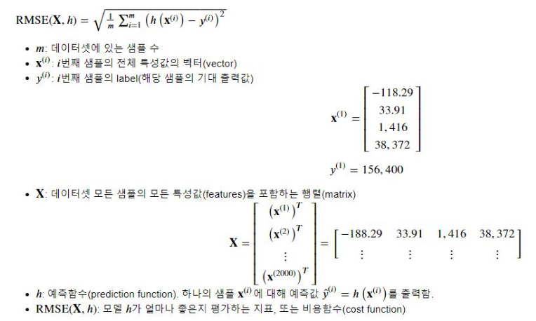
성능측정지표(performance measure) 선택
평균제곱근 오차(root mean square error(RMSE))
2. 데이터 가져오기(Get th Data)
- 작업환경 설정
# 윈도우는 아래 참조 (아래 링크 그대로 하였다.)
# https://github.com/ageron/handson-ml/issues/525
$ export ML_PATH="$HOME/ml" # You can change the path if you prefer
$ mkdir -p $ML_PATH

$ python3 -m pip --version
pip 19.3.1 from [...]/lib/python3.7/site-packages/pip (python 3.7)

$ python3 -m pip install --user -U pip
Collecting pip
[...]
Successfully installed pip-19.3.1- 독립적인 환경(isolated environment) 만들기
$ python3 -m pip install --user -U virtualenv
Collecting virtualenv
[...]
Successfully installed virtualenv-16.7.6

$ cd $ML_PATH
$ python3 -m virtualenv my_env
Using base prefix '[...]'
New python executable in [...]/ml/my_env/bin/python3
Also creating executable in [...]/ml/my_env/

$ cd $ML_PATH
$ source my_env/bin/activate # on Linux or macOS
$ .\my_env\Scripts\activate # on Windows- 필요한 패키지들 설치하기
$ python3 -m pip install -U jupyter matplotlib numpy pandas scipy scikit-learn
Collecting jupyter
Downloading https://[...]/jupyter-1.0.0-py2.py3-none-any.whl
Collecting matplotlib
[...]- 커널을 Jupyter에 등록하고 이름 정하기
$ python3 -m ipykernel install --user --name=python3- Jupyter 실행
$ jupyter notebook
[...] Serving notebooks from local directory: [...]/ml
[...] The Jupyter Notebook is running at:
[...] http://localhost:8888/?token=60995e108e44ac8d8865a[...]
[...] or http://127.0.0.1:8889/?token=60995e108e44ac8d8865a[...]
[...] Use Control-C to stop this server and shut down all kernels [...]
데이터 다운로드
# Python ≥3.5 is required
import sys
assert sys.version_info >= (3, 5)

# Scikit-Learn ≥0.20 is required
import sklearn
assert sklearn.__version__ >= "0.20"

# Common imports
import numpy as np
import os

# To plot pretty figures
%matplotlib inline
import matplotlib as mpl
import matplotlib.pyplot as plt
mpl.rc('axes', labelsize=14)
mpl.rc('xtick', labelsize=12)
mpl.rc('ytick', labelsize=12)

# Where to save the figures
PROJECT_ROOT_DIR = "."
CHAPTER_ID = "end_to_end_project"
IMAGES_PATH = os.path.join(PROJECT_ROOT_DIR, "images", CHAPTER_ID)
os.makedirs(IMAGES_PATH, exist_ok=True)

def save_fig(fig_id, tight_layout=True, fig_extension="png", resolution=300):
    path = os.path.join(IMAGES_PATH, fig_id + "." + fig_extension)
    print("Saving figure", fig_id)
    if tight_layout:
        plt.tight_layout()
    plt.savefig(path, format=fig_extension, dpi=resolution)

# Ignore useless warnings (see SciPy issue #5998)
import warnings
warnings.filterwarnings(action="ignore", message="^internal gelsd")
import os
import tarfile
import urllib
DOWNLOAD_ROOT = "https://raw.githubusercontent.com/ageron/handson-ml2/master/"
HOUSING_PATH = os.path.join("datasets", "housing")
HOUSING_URL = DOWNLOAD_ROOT + "datasets/housing/housing.tgz"
def fetch_housing_data(housing_url=HOUSING_URL, housing_path=HOUSING_PATH):
if not os.path.isdir(housing_path):
os.makedirs(housing_path)
tgz_path = os.path.join(housing_path, "housing.tgz")
urllib.request.urlretrieve(housing_url, tgz_path)
housing_tgz = tarfile.open(tgz_path)
housing_tgz.extractall(path=housing_path)
housing_tgz.close()fetch_housing_data()import pandas as pd
def load_housing_data(housing_path=HOUSING_PATH):
csv_path = os.path.join(housing_path, "housing.csv")
return pd.read_csv(csv_path)데이터 구조 훑어보기
housing = load_housing_data()
housing.head()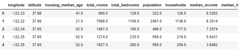
housing.info()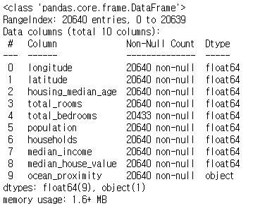
#ocean_proximity: 범주형(categorical) 필드
housing["ocean_proximity"].value_counts()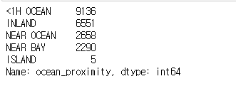
# describe(): 숫자형 특성의 정보를 요약
housing.describe()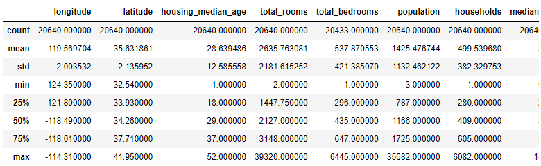
#히스토그램으로 데이터 분석해보기
%matplotlib inline
import matplotlib.pyplot as plt
housing.hist(bins=50, figsize=(20,15))
save_fig("attribute_histogram_plots")
plt.show()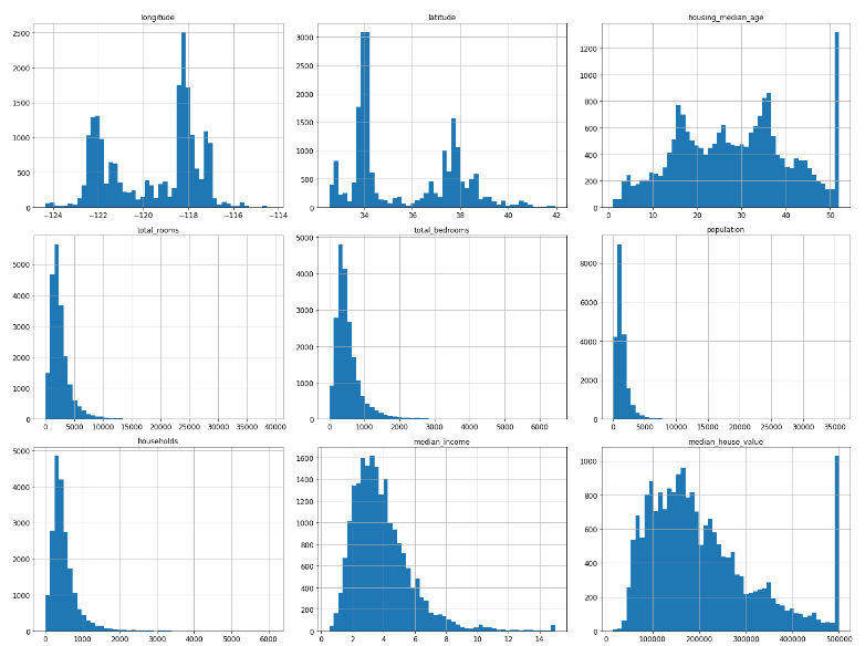
값이 이상하다면 만든 사람에게 물어보는 것이 중요하다.
테스트 데이터셋 만들기
좋은 모델을 만들기 위해선 훈련에 사용되지 않고 모델평가만을 위해서 사용될 "테스트 데이터셋"을 따로 구분하는 것이 필요하다. 테스트 데이터셋을 별도로 생성할 수도 있지만 프로젝트 초기의 경우 하나의 데이터셋을 훈련, 테스트용으로 분리하는 것이 일반적이다.
# to make this motebook's output identical at every run
np.random.seed(42)
import numpy as np
# For illustration only. Sklearn has train_test_split()
# 몇 퍼센트를 테스트 데이터로 사용할지 만드는 함수
def split_train_test(data, test_ratio):
shuffled_indices = np.random.permutation(len(data))
test_set_size = int(len(data) * test_ratio)
test_indices = shuffled_indices[:test_set_size]
train_indices = shuffled_indices[test_set_size:]
return data.iloc[train_indices], data.iloc[test_indices]a = np.random.permutation(10)
-> array([0, 1, 8, 5, 3, 4, 7, 9, 6, 2])# 80% train, 20% test
train_set, test_set = split_train_test(housing, 0.2)
len(train_set), len(test_set)
-> (16512, 4128)새로운 데이터가 들어왔을때 다시 한번 분리작업을 하게 된다. 이 작업에서 원하지 않는 데이터들이 섞이게 된다. 따라서 데이터의 유지를 위해서 샘플의 식별자를 사용하여 분할한다.
from zlib import crc32

# crc32: hashing 함수
def test_set_check(identifier, test_ratio):
    return crc32(np.int64(identifier)) & 0xffffffff < test_ratio * 2**32

def split_train_test_by_id(data, test_ratio, id_column):
    ids = data[id_column]
    in_test_set = ids.apply(lambda id_: test_set_check(id_, test_ratio))
    return data.loc[~in_test_set], data.loc[in_test_set]
# 인덱스를 id로 추가하기
housing_with_id = housing.reset_index() # adds an `index` column
train_set, test_set = split_train_test_by_id(housing_with_id, 0.2, "index")
housing_with_id.head()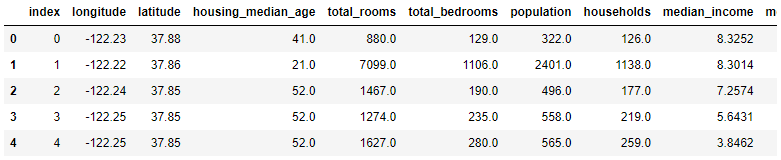
id가 행번호를 사용하게 되면 데이터가 변할 때 행 번호가 바뀌게 되는 문제가 발생한다. 따라서 id를 만드는데 안전한 feature를 사용한다.
# 위도와 경도를 feature로서 id를 만드는데 사용한다.
housing_with_id["id"] = housing["longitude"] * 1000 + housing["latitude"]
train_set, test_set = split_train_test_by_id(housing_with_id, 0.2, "id")
train_set.head()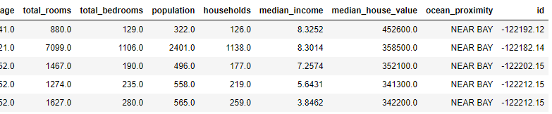
- Scikit-Learn에서 기본적으로 제공되는 데이터분할 함수
from sklearn.model_selection import train_test_split

train_set, test_set = train_test_split(housing, test_size=0.2, random_state=42)
계층적 샘플링(stratified sampling)
- 전체 데이터를 계층(stata)라는 동질의 그룹으로 나누고, 테스트 데이터가 전체 데이터를 잘 대표하도록 각 계층에서 올바른 수의 샘플을 추출
# 직관적으로 봤을 때 집의 가격은 수입과 비례할 것이라 생각
housing["median_income"].hist()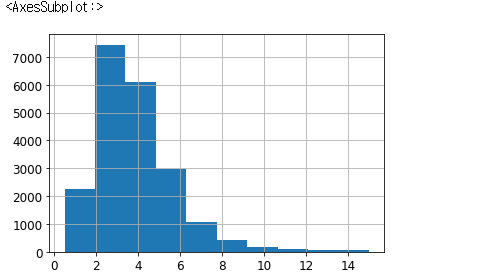
# pandas cut을 사용하면 grouping하기 편하다
housing["income_cat"] = pd.cut(housing["median_income"],
                               bins=[0., 1.5, 3.0, 4.5, 6., np.inf],
                               labels=[1, 2, 3, 4, 5])
housing["income_cat"].value_counts()

->3    7236
2    6581
4    3639
5    2362
1     822
Name: income_cat, dtype: int64
# 각각의 카테고리에 충분한 갯수로 분배되어야 한다.
housing["income_cat"].hist()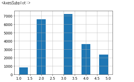
#scikit learn은 계층적 샘플링을 이미 제공한다.
from sklearn.model_selection import StratifiedShuffleSplit

split = StratifiedShuffleSplit(n_splits=1, test_size=0.2, random_state=42)
for train_index, test_index in split.split(housing, housing["income_cat"]):
    strat_train_set = housing.loc[train_index]
    strat_test_set = housing.loc[test_index]
strat_train_set.info()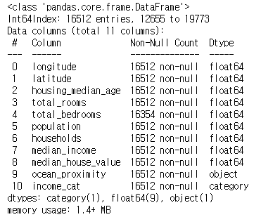
start_test_set.info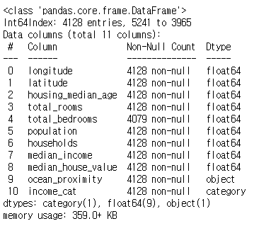
# 비율 확인
housing["income_cat"].value_counts() / len(housing)

->
3    0.350581
2    0.318847
4    0.176308
5    0.114438
1    0.039826
Name: income_cat, dtype: float64
# 비율이 유사함을 확인할 수 있다.
strat_test_set["income_cat"].value_counts() / len(strat_test_set)
->
3 0.350533
2 0.318798
4 0.176357
5 0.114341
1 0.039971
Name: income_cat, dtype: float64데이터 이해를 위한 탐색과 시각화
# 복사본 만들기
housing = strat_train_set.copy()
#지리적 데이터 시각화
housing.plot(kind="scatter", x="longitude", y="latitude")
save_fig("bad_visualization_plot")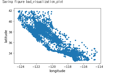
# 밀집된 영역 표시
# 알파옵션 사용
housing.plot(kind="scatter", x="longitude", y="latitude", alpha=0.1)
save_fig("better_visualization_plot")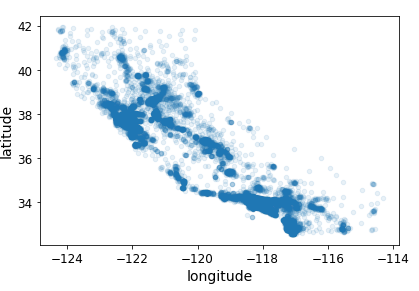
# 더 다양한 정보 표시
# s: 원의 반지름 => 인구
# c :  색상 -> 가격
housing.plot(kind='scatter', x='longitude', y='latitude', alpha=0.4,
            s=housing['population']/100, label='population', figsize=(10, 7),
            c = 'median_house_value', cmap=plt.get_cmap('jet'), colorbar=True, sharex=False)
plt.legend()
save_fig('housing_prices_scatterplot')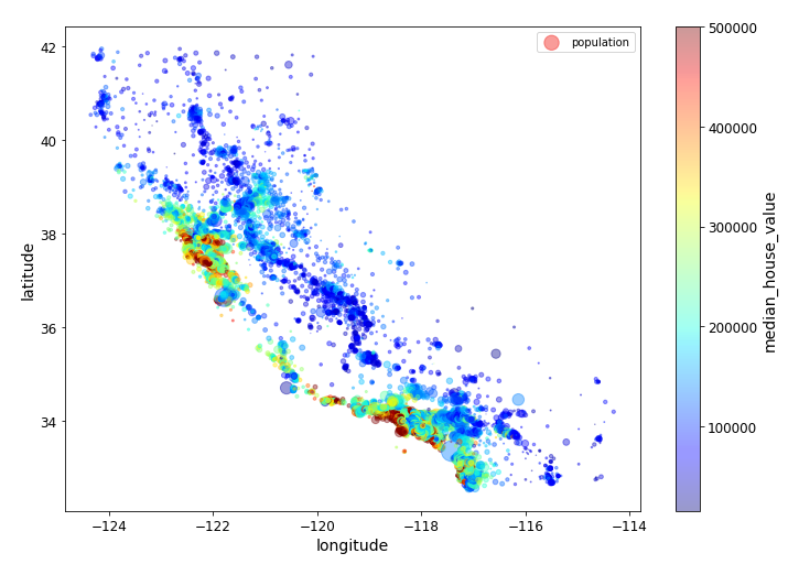
# Download the California image
image_path = os.path.join(PROJECT_ROOT_DIR, 'images', 'end_to_end_project')
os.makedirs(image_path, exist_ok=True)
DDOWNLOAD_ROOT = 'https://github.com/ageron/handson-ml2/blob/master/images/end_to_end_project/'
filename = "california.png"
import matplotlib.image as mpimg
california_img = mpimg.imread(os.path.join(image_path, filename))
ax = housing.plot(kind='scatter', x='longitude', y='latitude', figsize=(10, 8),
s = housing['population']/100, label='Population',
c = 'median_house_value', cmap=plt.get_cmap('jet'), colorbar=False, alpha=0.4)
plt.imshow(california_img, extent=[-124.55, -113.80, 32.45, 42.05], alpha=0.5, cmap=plt.get_cmap('jet'))
plt.xlabel('Latitude', fontsize=14)
plt.ylabel('Longitude', fontsize=14)
prices = housing['median_house_value']
tick_values = np.linspace(prices.min(), prices.max(), 11)
cbar = plt.colorbar()
cbar.ax.set_yticklabels(["$%dk"%(round(v/1000)) for v in tick_values], fontsize=14)
cbar.set_label('Median House Value', fontsize=16)
plt.legend()
save_fig('california_housing_prices_plot')
plt.show()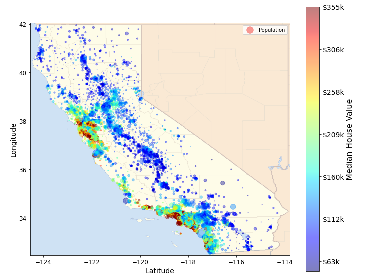
상관관계(Correlations) 관찰하기
corr_matrix = housing.corr()
# 1에 가까울 수록 상관관계가 있다.
# 음의 상관관계 -> latitude (북쪽으로 갈 수록 집 값이 내려간다라고 생각은 할 수 있다..?)
corr_matrix["median_house_value"].sort_values(ascending=False)

->
median_house_value    1.000000
median_income         0.688075
total_rooms           0.134153
housing_median_age    0.105623
households            0.065843
total_bedrooms        0.049686
population           -0.024650
longitude            -0.045967
latitude             -0.144160
Name: median_house_value, dtype: float64
scatter_matrix 사용해서 상관관계 확인하기
# from pandas.tools.plotting import scatter_matrix # for older version of pandas
from pandas.plotting import scatter_matrix

# 몇몇 특성만 확인
attributes = ['median_house_value', 'median_income', 'total_rooms', 'housing_median_age']
scatter_matrix(housing[attributes], figsize=(12, 8))
save_fig('scatter_matrix_plot')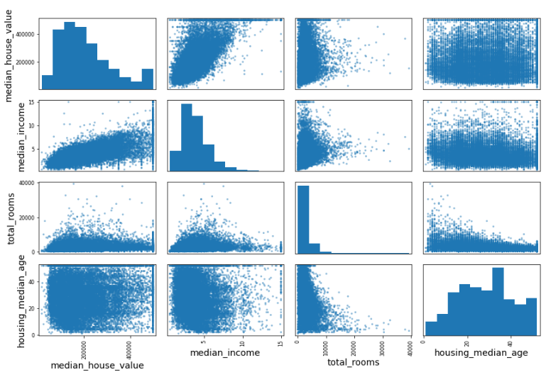
대각선에 있는 것은 자기 자신과 하는 것이므로 1이다.
# 확대해서 보기
housing.plot(kind='scatter', x='median_income', y='median_house_value', alpha=0.1)
plt.axis([0, 16, 0, 550000])
save_fig('income_vs_house_value_scatterplot')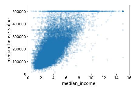
데이터를 시각화해서 살펴보면 데이터에 문제가 없는지를 발견하는데에 도움이 된다.
특성공학 실험
- 여러 특성(feature, attribute)들의 조합으로 새로운 특성을 정의해볼 수 있음
- 예를 들자면, 가구당 방 개수, 침대방(bedroom)의 비율, 가구당 인원
housing['rooms_per_household'] = housing['total_rooms']/housing['households']
housing['bedrooms_per_household'] = housing['total_bedrooms']/housing['total_rooms']
housing['population_per_household'] = housing['population']/housing['households']

# 집에 방이 많을 수록 비싸진다.
# 한 집에서 침실이 차지하는 비율은 집이 커질 수록 작아진다.
corr_matrix = housing.corr()
corr_matrix['median_house_value'].sort_values(ascending=False)

->
median_house_value          1.000000
median_income               0.688075
rooms_per_household         0.151948
total_rooms                 0.134153
housing_median_age          0.105623
households                  0.065843
total_bedrooms              0.049686
population_per_household   -0.023737
population                 -0.024650
longitude                  -0.045967
latitude                   -0.144160
bedrooms_per_household     -0.255880
Name: median_house_value, dtype: float64
머신러닝 알고리즘을 위한 데이터 준비
데이터 준비는 데이터 변환(data transformation)과정으로 볼 수 있다.
데이터 수동변환 vs. 자동변환(함수만들기)
데이터 자동변환의 장점들
1. 새로운 데이터에 대한 변환을 손쉽게 재생산(reproduce)할 수 있다.
2. 향후에 재사용(reuse)할 수 있는 라이브러리를 구축하게 된다.
3. 실제 시스템에서 가공되지 않은 데이터(raw data)를 알고리즘에 쉽게 입력으로 사용할 수 있도록 해준다.
4. 여러 데이터 변환 방법을 쉽게 시도해 볼 수 있다.
housing = strat_train_set.drop("median_house_value", axis=1) # drop labels for training set
housing_labels = strat_train_set["median_house_value"].copy()
데이터 정제(Data cleaning)
누락된 값(missing values) 다루는 방법들
1. 해당 구역을 제거(행을 제거)
2. 해당 특성을 제거(열을 제거)
3. 어떤 값으로 채움(0, 평균, 중간값 등)
housing.isnull().any(axis=1)

->
12655    False
15502    False
2908     False
14053    False
20496    False
         ...
15174    False
12661    False
19263    False
19140    False
19773    False
Length: 16512, dtype: bool
sample_incomplete_rows = housing[housing.isnull().any(axis=1)].head() # True if there is a null feature
sample_incomplete_rows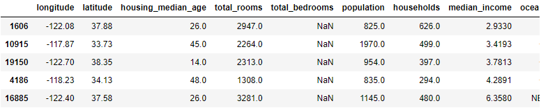
- 해당 구역 제거
sample_incomplete_rows.dropna(subset=['total_bedrooms']) # option1- 해당 특성을 제거
sample_incomplete_rows.drop("total_bedrooms", axis=1) # option 2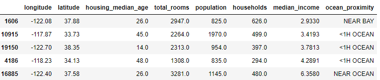
- 어떤 값으로 채움(0, 평균, 중간값 등)
median = housing["total_bedrooms"].median()
sample_incomplete_rows["total_bedrooms"].fillna(median, inplace=True) # option 3
sample_incomplete_rows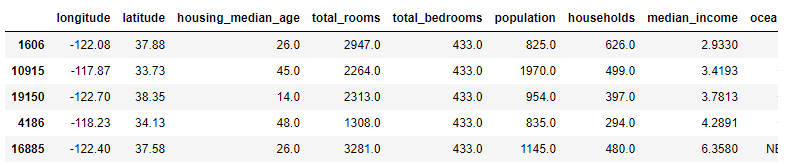
대부분의 경우는 채우거나 보전해주는 방향으로 사용한다.
SimpleImputer 사용하기
# 값이 없는 경우 중간 값으로 채우라.
from sklearn.impute import SimpleImputer
imputer = SimpleImputer(strategy="median")
# 중간값은 수치형 특성에서만 계산될 수 있기 때문에 텍스트 특성을 제외한 복사본을 생성
housing_num = housing.drop('ocean_proximity', axis=1)imputer.fit(housing_num)
->
SimpleImputer(strategy='median')# median 값 확인
imputer.statistics_
->
array([-118.51 , 34.26 , 29. , 2119. , 433. ,
1164. , 408. , 3.54155])# data frame 에서도 가능
housing_num.median().values
->
array([-118.51 , 34.26 , 29. , 2119. , 433. ,
1164. , 408. , 3.54155])이제 학습된 imputer 객체를 사용해 누락된 값을 중간값으로 바꿀 수 있다.
X = imputer.transform(housing_num)
X[0]

->
array([-1.2146e+02,  3.8520e+01,  2.9000e+01,  3.8730e+03,  7.9700e+02,
        2.2370e+03,  7.0600e+02,  2.1736e+00])
위 X는 NumPy array입니다. 이를 다시 pandas DataFrame으로 되돌릴 수 있다.
housing_tr = pd.DataFrame(X, columns=housing_num.columns, index=housing.index)제대로 채워져 있는지 확인해봅시다.
sample_incomplete_rows.index.values
housing_num.loc[sample_incomplete_rows.index.values]
housing_tr.loc[sample_incomplete_rows.index.values]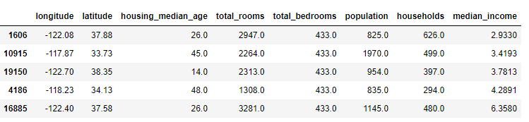
Estimator, Transformer, Predictor
-
추정기(estimator): 데이터셋을 기반으로 모델 파라미터들을 추정하는 객체를 추정기라고 한다(예를 들자면 imputer). 추정자체는 fit() method에 의해서 수행되고 하나의 데이터셋을 매개변수로 전달받는다(지도학습의 경우 label을 담고 있는 데이터셋을 추가적인 매개변수로 전달).
-
변환기(transformer): (imputer같이) 데이터셋을 변환하는 추정기를 변환기라고 한다. 변환은 transform() method가 수행한다. 그리고 변환된 데이터셋을 반환한다.
-
예측기(predictor): 일부 추정기는 주어진 새로운 데이터셋에 대해 예측값을 생성할 수 있다. 앞에서 사용했던 LinearRegression도 예측기이다. 예측기의 predict() method는 새로운 데이터셋을 받아 예측값을 반환한다. 그리고 score() method는 예측값에 대한 평가지표를 반환한다.
텍스트와 범주형 특성 다루기
housing_cat = housing[['ocean_proximity']]
housing_cat.head()

->
	ocean_proximity
12655	INLAND
15502	NEAR OCEAN
2908	INLAND
14053	NEAR OCEAN
20496	<1H OCEAN
대부분의 모델은 숫자를 input으로 받아들이기 때문에 텍스트를 numerical한 형태로 바꾸어주어야 한다.
# fit과 tranform을 한 번에 할 수 있다.
from sklearn.preprocessing import OrdinalEncoder

ordinal_encoder = OrdinalEncoder()
housing_cat_encoded = ordinal_encoder.fit_transform(housing_cat)
housing_cat_encoded[:10]

->
array([[1.],
       [4.],
       [1.],
       [4.],
       [0.],
       [3.],
       [0.],
       [0.],
       [0.],
[0.]])ordinal_encoder.categories_
->
[array(['<1H OCEAN', 'INLAND', 'ISLAND', 'NEAR BAY', 'NEAR OCEAN'],
dtype=object)]이 표현방식의 문제점
- "특성의 값이 비슷할수록 두 개의 샘플이 비슷하다"가 성립할 때 모델학습이 쉬워짐.
One-hot encoding
#sparse matrix
from sklearn.preprocessing import OneHotEncoder

cat_encoder = OneHotEncoder()
housing_cat_1hot = cat_encoder.fit_transform(housing_cat)


->
<16512x5 sparse matrix of type '<class 'numpy.float64'>'
	with 16512 stored elements in Compressed Sparse Row format>
위 출력을 보면 일반적인 배열이 아니고 "sparse matrix"임을 알 수 있다.
housing_cat_1hot.toarray()

->
array([[0., 1., 0., 0., 0.],
       [0., 0., 0., 0., 1.],
       [0., 1., 0., 0., 0.],
       ...,
       [1., 0., 0., 0., 0.],
       [1., 0., 0., 0., 0.],
       [0., 1., 0., 0., 0.]])
# 일반적인 array
cat_encoder = OneHotEncoder(sparse=False)
housing_cat_1hot = cat_encoder.fit_transform(housing_cat)
housing_cat_1hot

->
array([[0., 1., 0., 0., 0.],
       [0., 0., 0., 0., 1.],
       [0., 1., 0., 0., 0.],
       ...,
       [1., 0., 0., 0., 0.],
       [1., 0., 0., 0., 0.],
       [0., 1., 0., 0., 0.]])
-> one-hot encoding : 해당하는 위치만 1 나머지 다 0
나만의 변환기(Custom Transformers) 만들기
Scikit-Learn이 유용한 변환기를 많이 제공하지만 프로젝트를 위해 특별한 데이터 처리 작업을 해야 할 경우가 많다. 이 때 나만의 변환기를 만들 수 있다.
반드시 구현해야 할 method들
1. fit()
2. transform()
아래의 custom tranformer는 rooms_per_household, population_per_household 두 개의 새로운 특성을 데이터셋에 추가하며 add_bedrooms_per_room = True로 주어지면 bedrooms_per_room 특성까지 추가합니다. add_bedrooms_per_room은 하이퍼파라미터.
from sklearn.base import BaseEstimator, TransformerMixin

# column index
rooms_ix, bedrooms_ix, population_ix, households_ix = 3, 4, 5, 6

class CombinedAttributesAdder(BaseEstimator, TransformerMixin):
    def __init__(self, add_bedrooms_per_room = True): # no *args or **kargs
        self.add_bedrooms_per_room = add_bedrooms_per_room
    def fit(self, X, y=None):
        return self  # nothing else to do
    def transform(self, X):
        rooms_per_household = X[:, rooms_ix] / X[:, households_ix]
        population_per_household = X[:, population_ix] / X[:, households_ix]
        if self.add_bedrooms_per_room:
            bedrooms_per_room = X[:, bedrooms_ix] / X[:, rooms_ix]
            return np.c_[X, rooms_per_household, population_per_household,
                         bedrooms_per_room]
        else:
            return np.c_[X, rooms_per_household, population_per_household]

attr_adder = CombinedAttributesAdder(add_bedrooms_per_room=False)
housing_extra_attribs = attr_adder.transform(housing.values)
Numpy데이터를 DataFrame으로 변환
housing_extra_attribs = pd.DataFrame(
    housing_extra_attribs,
    columns=list(housing.columns)+["rooms_per_household", "population_per_household"],
    index=housing.index)
housing_extra_attribs.head()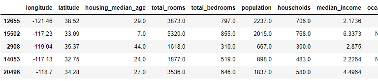
특성 스케일링
- Min-max scaling: 0과 1 사이의 값이 되도록 조정
- 표준화(standardization): 평균이 0, 분산이 1이 되도록 만들어 준다.(sklearn StandardScaler를 사용)
변환 파이프라인(Transformation Pipelines)
여러 개의 변환이 순차적으로 이루어져야 할 경우 Pipeline class를 사용하면 편하다.
from sklearn.pipeline import Pipeline
from sklearn.preprocessing import StandardScaler

num_pipeline = Pipeline([
        ('imputer', SimpleImputer(strategy="median")),
        ('attribs_adder', CombinedAttributesAdder()),
        ('std_scaler', StandardScaler()),
    ])

housing_num_tr = num_pipeline.fit_transform(housing_num)
이름, 추정기 쌍의 목록
마지막 단계를 제외하고 모두 변환기여야 한다(fit_transform() method를 가지고 있어야 함).
파이프라인의 fit() method를 호출하면 모든 변환기의 fit_transform() method를 순서대로 호출하면서 한 단계의 출력을 다음 단계의 입력으로 전달한다. 마지막 단계에서는 fit() method만 호출한다.
housing_num_tr

->
array([[-0.94135046,  1.34743822,  0.02756357, ...,  0.01739526,
         0.00622264, -0.12112176],
       [ 1.17178212, -1.19243966, -1.72201763, ...,  0.56925554,
        -0.04081077, -0.81086696],
       [ 0.26758118, -0.1259716 ,  1.22045984, ..., -0.01802432,
        -0.07537122, -0.33827252],
       ...,
       [-1.5707942 ,  1.31001828,  1.53856552, ..., -0.5092404 ,
        -0.03743619,  0.32286937],
       [-1.56080303,  1.2492109 , -1.1653327 , ...,  0.32814891,
        -0.05915604, -0.45702273],
       [-1.28105026,  2.02567448, -0.13148926, ...,  0.01407228,
         0.00657083, -0.12169672]])
각 열(column) 마다 다른 파이프라인을 적용할 수도 있다! 예를 들어 수치형 특성들과 범주형 특성들에 대해 별도의 변환이 필요하다면 아래와 같이 ColumnTransformer를 사용하면 된다.
from sklearn.compose import ColumnTransformer

num_attribs = list(housing_num)
cat_attribs = ['ocean_proximity']

full_pipeline = ColumnTransformer([
    ('num', num_pipeline, num_attribs),
    ('cat', OneHotEncoder(), cat_attribs),
])

housing_prepared = full_pipeline.fit_transform(housing)
housing_prepared
->
array([[-0.94135046, 1.34743822, 0.02756357, ..., 0. ,
0. , 0. ],
[ 1.17178212, -1.19243966, -1.72201763, ..., 0. ,
0. , 1. ],
[ 0.26758118, -0.1259716 , 1.22045984, ..., 0. ,
0. , 0. ],
...,
[-1.5707942 , 1.31001828, 1.53856552, ..., 0. ,
0. , 0. ],
[-1.56080303, 1.2492109 , -1.1653327 , ..., 0. ,
0. , 0. ],
[-1.28105026, 2.02567448, -0.13148926, ..., 0. ,
0. , 0. ]])
housing_prepared.shape, housing.shape
->
((16512, 16), (16512, 9))모델 훈련(Train a Model)
드디어 모델을 훈련시킬 준비가 되었다! 지난 시간에 배웠던 선형회귀모델(linear regression)을 사용해보자.
from sklearn.linear_model import LinearRegression
#인스턴스 형성
lin_reg = LinearRegression()
lin_reg.fit(housing_prepared, housing_labels)
모델훈련은 딱 3줄의 코드면 충분하다!
몇 개의 샘플에 모델을 적용해서 예측값을 확인해보고 실제값과 비교해보자.
lin_reg.coef_

->
array([-55649.63398453, -56711.59742892,  13734.72084192,  -1943.05586355,
         7343.22979731, -45709.28253579,  45453.26277662,  74714.15226133,
         6604.58396628,   1043.05452981,   9248.31607777, -18015.98870784,
       -55214.71083473, 110357.8461062 , -22484.65997391, -14642.48658971])
#계수의 절대값이 클수록 영향력이 크다.
# 계수값이 작은 경우 영향이 없는 것은 아니다.
# feature들 가운데 몇 가지는 겹치는 경우가 있어 그 중 하나만 큰 값을 가지는 경우도 있다.
# 크기만 가지고 중요성을 판단하는 것은 위험하다.
# 계수값에 따라서 어떻게 모델에 영향을 미치는 지 확인
extra_attribs = ['rooms_per_hhold', 'pop_per_hhold', 'bedrooms_per_room']
cat_encoder = full_pipeline.named_transformers_['cat']
cat_one_hot_attribs = list(cat_encoder.categories_[0])
attributes = num_attribs + extra_attribs + cat_one_hot_attribs
sorted(zip(lin_reg.coef_, attributes), reverse=True)
->
[(110357.84610619607, 'ISLAND'),
(74714.15226132619, 'median_income'),
(45453.262776622236, 'households'),
(13734.720841922466, 'housing_median_age'),
(9248.31607776975, 'bedrooms_per_room'),
(7343.229797309003, 'total_bedrooms'),
(6604.583966284028, 'rooms_per_hhold'),
(1043.0545298050245, 'pop_per_hhold'),
(-1943.0558635496077, 'total_rooms'),
(-14642.48658971256, 'NEAR OCEAN'),
(-18015.98870783896, '<1H OCEAN'),
(-22484.659973912247, 'NEAR BAY'),
(-45709.28253579062, 'population'),
(-55214.71083473229, 'INLAND'),
(-55649.63398452769, 'longitude'),
(-56711.597428916226, 'latitude')]# 5개의 샘플에 대해 데이터변환 및 예측을 해보자
some_data = housing.iloc[:5]
some_labels = housing_labels.iloc[:5]
some_data_prepared = full_pipeline.transform(some_data)
print("Predictions:", lin_reg.predict(some_data_prepared).round(decimals=1))
->
Predictions: [ 85657.9 305492.6 152056.5 186095.7 244550.7]
# 주어진 label 값 확인
print("Labels:", list(some_labels))
->
Labels: [72100.0, 279600.0, 82700.0, 112500.0, 238300.0]전체 훈련 데이터셋에 대한 RMSE를 측정
from sklearn.metrics import mean_squared_error

housing_predictions = lin_reg.predict(housing_prepared)
lin_mse = mean_squared_error(housing_labels, housing_predictions)
lin_rmse = np.sqrt(lin_mse)
lin_rmse
->
68627.87390018745
훈련 데이터셋의 RMSE가 이 경우처럼 큰 경우 => 과소적합(under-fitting)
과소적합이 일어나는 이유?
1. 특성들(features)이 충분한 정보를 제공하지 못함
2. 모델이 충분히 강력하지 못함
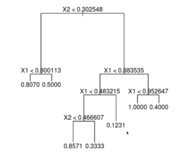
강력한 비선형모델인 DecisionTreeRegressor를 사용
# 학습
from sklearn.tree import DecisionTreeRegressor

tree_reg = DecisionTreeRegressor(random_state=42)
tree_reg.fit(housing_prepared, housing_labels)
# 과잉 적합일 경우가 높다.
housing_predictions = tree_reg.predict(housing_prepared)
tree_mse = mean_squared_error(housing_labels, housing_predictions)
tree_rmse = np.sqrt(tree_mse)
tree_rmse
->
0.0이 모델이 선형모델보다 낫다고 말할 수 있을까? 어떻게 알 수 있을까?
- 테스트 데이터셋을 이용한 검증
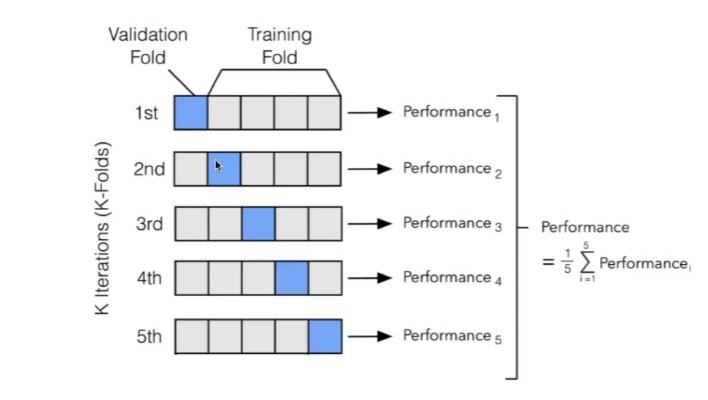
(-> 추천x, 여러번 테스트 데이터를 보게 되면 학습모델에 영향을 미치게 된다. 가능하면 테스트 데이터는 모델을 론칭 직전까지 미루는 것이 좋다.) - 훈련 데이터셋의 일부를 검증데이터(validation data)셋으로 분리해서 검증
- k-겹 교차 검증(k-fold cross-validation)
교차 검증(Cross-Validation)을 사용한 평가
결정트리 모델에 대한 평가
# mean squared error에 -1 곱한 값 사용,
# 에러가 낮으면 낮을 수록 좋은 것이므로 값이 크게 나오면 작게 확인 할 수 있게.
from sklearn.model_selection import cross_val_score

scores = cross_val_score(tree_reg, housing_prepared, housing_labels,
                         scoring="neg_mean_squared_error", cv=10)

# 다시 값을 구하기 위해 scores에 -를 붙인다.
tree_rmse_scores = np.sqrt(-scores)
def display_scores(scores):
print("Scores:", scores)
print("Mean:", scores.mean())
print("Standard deviation:", scores.std())
display_scores(tree_rmse_scores)
->
Scores: [72831.45749112 69973.18438322 69528.56551415 72517.78229792
69145.50006909 79094.74123727 68960.045444 73344.50225684
69826.02473916 71077.09753998]
Mean: 71629.89009727491
Standard deviation: 2914.035468468928선형회귀모델에 대한 평가
lin_scores = cross_val_score(lin_reg, housing_prepared, housing_labels,
                             scoring="neg_mean_squared_error", cv=10)
lin_rmse_scores = np.sqrt(-lin_scores)
display_scores(lin_rmse_scores)

#mean이 트리보다 작다 -> 다음 새로운 데이터가 들어왔을 때 더 잘 할 확률이 높다.
->
Scores: [71762.76364394 64114.99166359 67771.17124356 68635.19072082
 66846.14089488 72528.03725385 73997.08050233 68802.33629334
 66443.28836884 70139.79923956]
Mean: 69104.07998247063
Standard deviation: 2880.3282098180666
RandomForestRegressor에 대한 평가
여러 개 트리 사용
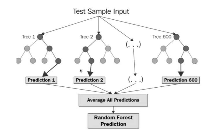
# 트리 100개 사용
from sklearn.ensemble import RandomForestRegressor

forest_reg = RandomForestRegressor(n_estimators=100, random_state=42)
forest_reg.fit(housing_prepared, housing_labels)
# 학습 데이터에 대한 에러
housing_predictions = forest_reg.predict(housing_prepared)
forest_mse = mean_squared_error(housing_labels, housing_predictions)
forest_rmse = np.sqrt(forest_mse)
forest_rmse
->
18650.698705770003from sklearn.model_selection import cross_val_score
forest_scores = cross_val_score(forest_reg, housing_prepared, housing_labels,
scoring="neg_mean_squared_error", cv=10)
forest_rmse_scores = np.sqrt(-forest_scores)
display_scores(forest_rmse_scores)
->
Scores: [51559.63379638 48737.57100062 47210.51269766 51875.21247297
47577.50470123 51863.27467888 52746.34645573 50065.1762751
48664.66818196 54055.90894609]
Mean: 50435.58092066179
Standard deviation: 2203.3381412764606모델 세부 튜닝(Fine-Tune Your Model)
모델의 종류를 선택한 후에 모델을 세부 튜닝하는 것이 필요하다. 모델 학습을 위한 최적의 하이퍼파라미터를 찾는 과정이라고 말할 수 있다.
그리드 탐색(Grid Search)
수동으로 하이퍼파라미터 조합을 시도하는 대신 Scikit learn에서 제공하는 GridSearchCV를 사용하는 것이 좋다.
from sklearn.model_selection import GridSearchCV

param_grid = [
    # try 12 (3×4) combinations of hyperparameters
    # 조합
    {'n_estimators': [3, 10, 30], 'max_features': [2, 4, 6, 8]},
    # then try 6 (2×3) combinations with bootstrap set as False
    # 18가지 조합
    {'bootstrap': [False], 'n_estimators': [3, 10], 'max_features': [2, 3, 4]},
  ]

forest_reg = RandomForestRegressor(random_state=42)
# train across 5 folds, that's a total of (12+6)*5=90 rounds of training
grid_search = GridSearchCV(forest_reg, param_grid, cv=5,
                           scoring='neg_mean_squared_error',
                           return_train_score=True)
grid_search.fit(housing_prepared, housing_labels)

->
GridSearchCV(cv=5, estimator=RandomForestRegressor(random_state=42),
             param_grid=[{'max_features': [2, 4, 6, 8],
                          'n_estimators': [3, 10, 30]},
                         {'bootstrap': [False], 'max_features': [2, 3, 4],
                          'n_estimators': [3, 10]}],
             return_train_score=True, scoring='neg_mean_squared_error')
# 가장 좋은 모델을 만드는 조합
grid_search.best_params_
->
{'max_features': 8, 'n_estimators': 30}
grid_search.best_estimator_
->
RandomForestRegressor(max_features=8, n_estimators=30, random_state=42)# 조합에 따라 어떻게 바뀌는지 확인 가능
cvres = grid_search.cv_results_
for mean_score, params in zip(cvres["mean_test_score"], cvres["params"]):
print(np.sqrt(-mean_score), params)
->
63895.161577951665 {'max_features': 2, 'n_estimators': 3}
54916.32386349543 {'max_features': 2, 'n_estimators': 10}
52885.86715332332 {'max_features': 2, 'n_estimators': 30}
60075.3680329983 {'max_features': 4, 'n_estimators': 3}
52495.01284985185 {'max_features': 4, 'n_estimators': 10}
50187.24324926565 {'max_features': 4, 'n_estimators': 30}
58064.73529982314 {'max_features': 6, 'n_estimators': 3}
51519.32062366315 {'max_features': 6, 'n_estimators': 10}
49969.80441627874 {'max_features': 6, 'n_estimators': 30}
58895.824998155826 {'max_features': 8, 'n_estimators': 3}
52459.79624724529 {'max_features': 8, 'n_estimators': 10}
49898.98913455217 {'max_features': 8, 'n_estimators': 30}
62381.765106921855 {'bootstrap': False, 'max_features': 2, 'n_estimators': 3}
54476.57050944266 {'bootstrap': False, 'max_features': 2, 'n_estimators': 10}
59974.60028085155 {'bootstrap': False, 'max_features': 3, 'n_estimators': 3}
52754.5632813202 {'bootstrap': False, 'max_features': 3, 'n_estimators': 10}
57831.136061214274 {'bootstrap': False, 'max_features': 4, 'n_estimators': 3}
51278.37877140253 {'bootstrap': False, 'max_features': 4, 'n_estimators': 10}랜덤 탐색(Randomized Search)
하이퍼파라미터 조합의 수가 큰 경우에 유리. 지정한 횟수만큼만 평가.
from sklearn.model_selection import RandomizedSearchCV
from scipy.stats import randint

param_distribs = {
        'n_estimators': randint(low=1, high=200),
        'max_features': randint(low=1, high=8),
    }

forest_reg = RandomForestRegressor(random_state=42)
rnd_search = RandomizedSearchCV(forest_reg, param_distributions=param_distribs,
                                n_iter=10, cv=5, scoring='neg_mean_squared_error', random_state=42)
rnd_search.fit(housing_prepared, housing_labels)

->
RandomizedSearchCV(cv=5, estimator=RandomForestRegressor(random_state=42),
                   param_distributions={'max_features': <scipy.stats._distn_infrastructure.rv_frozen object at 0x000001DF58D6FCC8>,
                                        'n_estimators': <scipy.stats._distn_infrastructure.rv_frozen object at 0x000001DF58D74C48>},
                   random_state=42, scoring='neg_mean_squared_error')
cvres = rnd_search.cv_results_
for mean_score, params in zip(cvres["mean_test_score"], cvres["params"]):
print(np.sqrt(-mean_score), params)
->
49117.55344336652 {'max_features': 7, 'n_estimators': 180}
51450.63202856348 {'max_features': 5, 'n_estimators': 15}
50692.53588182537 {'max_features': 3, 'n_estimators': 72}
50783.614493515 {'max_features': 5, 'n_estimators': 21}
49162.89877456354 {'max_features': 7, 'n_estimators': 122}
50655.798471042704 {'max_features': 3, 'n_estimators': 75}
50513.856319990606 {'max_features': 3, 'n_estimators': 88}
49521.17201976928 {'max_features': 5, 'n_estimators': 100}
50302.90440763418 {'max_features': 3, 'n_estimators': 150}
65167.02018649492 {'max_features': 5, 'n_estimators': 2}특성 중요도, 에러 분석
feature_importances = grid_search.best_estimator_.feature_importances_
feature_importances

->
array([6.96542523e-02, 6.04213840e-02, 4.21882202e-02, 1.52450557e-02,
       1.55545295e-02, 1.58491147e-02, 1.49346552e-02, 3.79009225e-01,
       5.47789150e-02, 1.07031322e-01, 4.82031213e-02, 6.79266007e-03,
       1.65706303e-01, 7.83480660e-05, 1.52473276e-03, 3.02816106e-03])
feature들과 연결해서 출력
extra_attribs = ["rooms_per_hhold", "pop_per_hhold", "bedrooms_per_room"]
#cat_encoder = cat_pipeline.named_steps["cat_encoder"] # old solution
cat_encoder = full_pipeline.named_transformers_["cat"]
cat_one_hot_attribs = list(cat_encoder.categories_[0])
attributes = num_attribs + extra_attribs + cat_one_hot_attribs
sorted(zip(feature_importances, attributes), reverse=True)

->
[(0.3790092248170967, 'median_income'),
 (0.16570630316895876, 'INLAND'),
 (0.10703132208204355, 'pop_per_hhold'),
 (0.06965425227942929, 'longitude'),
 (0.0604213840080722, 'latitude'),
 (0.054778915018283726, 'rooms_per_hhold'),
 (0.048203121338269206, 'bedrooms_per_room'),
 (0.04218822024391753, 'housing_median_age'),
 (0.015849114744428634, 'population'),
 (0.015554529490469328, 'total_bedrooms'),
 (0.01524505568840977, 'total_rooms'),
 (0.014934655161887772, 'households'),
 (0.006792660074259966, '<1H OCEAN'),
 (0.0030281610628962747, 'NEAR OCEAN'),
 (0.0015247327555504937, 'NEAR BAY'),
 (7.834806602687504e-05, 'ISLAND')]
테스트 데이터셋으로 최종 평가하기
#모델 선정 완료
final_model = grid_search.best_estimator_

X_test = strat_test_set.drop("median_house_value", axis=1)
y_test = strat_test_set["median_house_value"].copy()

X_test_prepared = full_pipeline.transform(X_test)
final_predictions = final_model.predict(X_test_prepared)

final_mse = mean_squared_error(y_test, final_predictions)
final_rmse = np.sqrt(final_mse)

final_rmse
->
47873.26095812988
론칭, 모니터링, 시스템 유지보수
상용환경에 배포하기 위해서 데이터 전처리와 모델의 예측이 포함된 파이프라인을 만들어 저장하는 것이 좋다.
# 변환과 예측 하나로
full_pipeline_with_predictor = Pipeline([
        ("preparation", full_pipeline),
        ("linear", LinearRegression())
    ])

full_pipeline_with_predictor.fit(housing, housing_labels)
full_pipeline_with_predictor.predict(some_data)

->
array([ 85657.90192014, 305492.60737488, 152056.46122456, 186095.70946094,
       244550.67966089])
my_model = full_pipeline_with_predictor
import joblib
joblib.dump(my_model, "my_model.pkl")
#...
my_model_loaded = joblib.load("my_model.pkl")
my_model_loaded.predict(some_data)
->
array([ 85657.90192014, 305492.60737488, 152056.46122456, 186095.70946094,
244550.67966089])론칭 후 시스템 모니터링
-
시간이 지나면 모델이 낙후되면서 성능이 저하
-
자동모니터링: 추천시스템의 경우, 추천된 상품의 판매량이 줄어드는지?
-
수동모니터링: 이미지 분류의 경우, 분류된 이미지들 중 일부를 전문가에게 검토시킴
-
결과가 나빠진 경우
-> 데이터 입력의 품질이 나빠졌는지? 센서고장?
-> 트렌드의 변화? 계절적 요인?유지보수
-
정기적으로 새로운 데이터 수집(레이블)
-
새로운 데이터를 테스트 데이터로, 현재의 테스트 데이터는 학습데이터로 편입
-
다시 학습후, 새로운 테스트 데이터에 기반해 현재 모델과 새 모델을 평가, 비교
전체 프로세스에 고르게 시간을 배분해야 한다.!