과적합을 막기 위해 정규화를 해보자
준비
# import packages
import numpy as np
import matplotlib.pyplot as plt
import sklearn
import sklearn.datasets
import scipy.io
from reg_utils import sigmoid, relu, plot_decision_boundary, initialize_parameters, load_2D_dataset, predict_dec
from reg_utils import compute_cost, predict, forward_propagation, backward_propagation, update_parameters
from testCases import *
from public_tests import *

%matplotlib inline
plt.rcParams['figure.figsize'] = (7.0, 4.0) # set default size of plots
plt.rcParams['image.interpolation'] = 'nearest'
plt.rcParams['image.cmap'] = 'gray'

%load_ext autoreload
%autoreload 2

# Loading the Dataset
train_X, train_Y, test_X, test_Y = load_2D_dataset()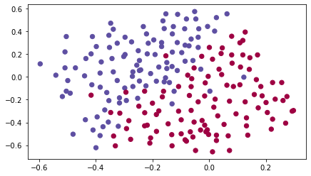
Non-Regularized Model
lambd를 nonzero로 설정해서 정규화 모드를 켠다.
keep_prob을 1보다 작은 값으로 설정해서 드롭아웃 모드를 켠다.
먼저 모델을 정규화 없이 실행해본 뒤,
- L2 :
"compute_cost_with_regularization()" and "backward_propagation_with_regularization()" - Dropout :
"forward_propagation_with_dropout()" and "backward_propagation_with_dropout()"
위 두 가지를 구현해보자
def model(X, Y, learning_rate = 0.3, num_iterations = 30000, print_cost = True, lambd = 0, keep_prob = 1):
    """
    Implements a three-layer neural network: LINEAR->RELU->LINEAR->RELU->LINEAR->SIGMOID.

    Arguments:
    X -- input data, of shape (input size, number of examples)
    Y -- true "label" vector (1 for blue dot / 0 for red dot), of shape (output size, number of examples)
    learning_rate -- learning rate of the optimization
    num_iterations -- number of iterations of the optimization loop
    print_cost -- If True, print the cost every 10000 iterations
    lambd -- regularization hyperparameter, scalar
    keep_prob - probability of keeping a neuron active during drop-out, scalar.

    Returns:
    parameters -- parameters learned by the model. They can then be used to predict.
    """

    grads = {}
    costs = []                            # to keep track of the cost
    m = X.shape[1]                        # number of examples
    layers_dims = [X.shape[0], 20, 3, 1]

    # Initialize parameters dictionary.
    parameters = initialize_parameters(layers_dims)

    # Loop (gradient descent)

    for i in range(0, num_iterations):

        # Forward propagation: LINEAR -> RELU -> LINEAR -> RELU -> LINEAR -> SIGMOID.
        if keep_prob == 1:
            a3, cache = forward_propagation(X, parameters)
        elif keep_prob < 1:
            a3, cache = forward_propagation_with_dropout(X, parameters, keep_prob)

        # Cost function
        if lambd == 0:
            cost = compute_cost(a3, Y)
        else:
            cost = compute_cost_with_regularization(a3, Y, parameters, lambd)

        # Backward propagation.
        assert (lambd == 0 or keep_prob == 1)   # it is possible to use both L2 regularization and dropout,
                                                # but this assignment will only explore one at a time
        if lambd == 0 and keep_prob == 1:
            grads = backward_propagation(X, Y, cache)
        elif lambd != 0:
            grads = backward_propagation_with_regularization(X, Y, cache, lambd)
        elif keep_prob < 1:
            grads = backward_propagation_with_dropout(X, Y, cache, keep_prob)

        # Update parameters.
        parameters = update_parameters(parameters, grads, learning_rate)

        # Print the loss every 10000 iterations
        if print_cost and i % 10000 == 0:
            print("Cost after iteration {}: {}".format(i, cost))
        if print_cost and i % 1000 == 0:
            costs.append(cost)

    # plot the cost
    plt.plot(costs)
    plt.ylabel('cost')
    plt.xlabel('iterations (x1,000)')
    plt.title("Learning rate =" + str(learning_rate))
    plt.show()

    return parameters
정규화 없는 모델을 실행시켜보자
parameters = model(train_X, train_Y)
print ("On the training set:")
predictions_train = predict(train_X, train_Y, parameters)
print ("On the test set:")
predictions_test = predict(test_X, test_Y, parameters)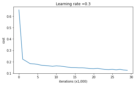
On the training set:
Accuracy: 0.9478672985781991
On the test set:
Accuracy: 0.915
위 결과를 베이스라인 삼아 정규화가 주는 영향을 알아볼 것이다.
plt.title("Model without regularization")
axes = plt.gca()
axes.set_xlim([-0.75,0.40])
axes.set_ylim([-0.75,0.65])
plot_decision_boundary(lambda x: predict_dec(parameters, x.T), train_X, train_Y)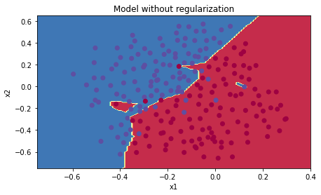
데이터의 노이즈 부분을 과적합하고 있다.
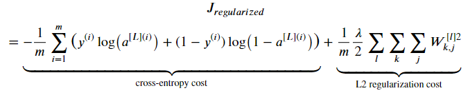
L2 Regularization
From:
To:
compute_cost_with_regularization
# GRADED FUNCTION: compute_cost_with_regularization

def compute_cost_with_regularization(A3, Y, parameters, lambd):
    """
    Implement the cost function with L2 regularization. See formula (2) above.

    Arguments:
    A3 -- post-activation, output of forward propagation, of shape (output size, number of examples)
    Y -- "true" labels vector, of shape (output size, number of examples)
    parameters -- python dictionary containing parameters of the model

    Returns:
    cost - value of the regularized loss function (formula (2))
    """
    m = Y.shape[1]
    W1 = parameters["W1"]
    W2 = parameters["W2"]
    W3 = parameters["W3"]

    cross_entropy_cost = compute_cost(A3, Y) # This gives you the cross-entropy part of the cost

L2_regularization_cost = (np.sum(np.square(W1))+np.sum(np.square(W2))+np.sum(np.square(W3))) * lambd / (2*m)

    cost = cross_entropy_cost + L2_regularization_cost

    return cost
backward_propagation_with_regularization
# GRADED FUNCTION: backward_propagation_with_regularization

def backward_propagation_with_regularization(X, Y, cache, lambd):
    """
    Implements the backward propagation of our baseline model to which we added an L2 regularization.

    Arguments:
    X -- input dataset, of shape (input size, number of examples)
    Y -- "true" labels vector, of shape (output size, number of examples)
    cache -- cache output from forward_propagation()
    lambd -- regularization hyperparameter, scalar

    Returns:
    gradients -- A dictionary with the gradients with respect to each parameter, activation and pre-activation variables
    """

    m = X.shape[1]
    (Z1, A1, W1, b1, Z2, A2, W2, b2, Z3, A3, W3, b3) = cache

    dZ3 = A3 - Y
    #(≈ 1 lines of code)
    # dW3 = 1./m * np.dot(dZ3, A2.T) + None
    # YOUR CODE STARTS HERE

    dW3 = 1./m * np.dot(dZ3, A2.T) + lambd * W3 / m

    # YOUR CODE ENDS HERE
    db3 = 1. / m * np.sum(dZ3, axis=1, keepdims=True)

    dA2 = np.dot(W3.T, dZ3)
    dZ2 = np.multiply(dA2, np.int64(A2 > 0))

    dW2 = 1./m * np.dot(dZ2, A1.T) + lambd * W2 / m #정규화항을 더해준다
    db2 = 1. / m * np.sum(dZ2, axis=1, keepdims=True)

    dA1 = np.dot(W2.T, dZ2)
    dZ1 = np.multiply(dA1, np.int64(A1 > 0))

    dW1 = 1./m * np.dot(dZ1, X.T) + lambd * W1 / m #정규화항을 더해준다
    db1 = 1. / m * np.sum(dZ1, axis=1, keepdims=True)

    gradients = {"dZ3": dZ3, "dW3": dW3, "db3": db3,"dA2": dA2,
                 "dZ2": dZ2, "dW2": dW2, "db2": db2, "dA1": dA1,
                 "dZ1": dZ1, "dW1": dW1, "db1": db1}

    return gradients
기존의 dW에 정규화항 을 더해주었다.
로 설정하고 L2 정규화 모델을 실행시켜보자
parameters = model(train_X, train_Y, lambd = 0.7)
print ("On the train set:")
predictions_train = predict(train_X, train_Y, parameters)
print ("On the test set:")
predictions_test = predict(test_X, test_Y, parameters)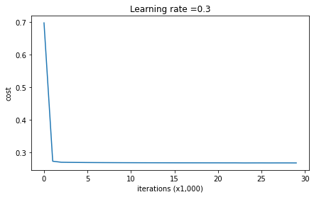
On the train set:
Accuracy: 0.9383886255924171
On the test set:
Accuracy: 0.93
정규화가 없을 때에 비해, 테스트세트의 정확도가 올랐다.
plt.title("Model with L2-regularization")
axes = plt.gca()
axes.set_xlim([-0.75,0.40])
axes.set_ylim([-0.75,0.65])
plot_decision_boundary(lambda x: predict_dec(parameters, x.T), train_X, train_Y)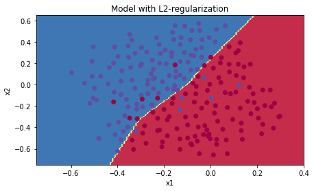
더이상 과적합도 일어나지 않는다.
𝜆의 값은 개발 세트(dev set)를 사용해 조정할 수 있는 하이퍼파라미터이다.
L2 정규화는 경계를 더 부드럽게 만든다. 그러나 𝜆값이 너무 크면 "oversmooth"되어 고편향 모델이 될 수도 있다.
✅비용 계산에 L2를 적용하면, 정규화항이 비용에 추가된다
✅BP함수에 L2를 적용하면, 가중치 행렬 w에 대한 항이 gradient에 추가된다
✅가중치는 점점 작아지게 된다 (weight decay)
Dropout Regularization
드롭아웃은 딥러닝에 많이 사용되는 정규화 기법으로, 매 반복마다 무작위로 일부 뉴런을 비활성화한다.
forward_propagation_with_dropout
1, 2번째 은닉층에 드롭아웃을 추가한다. 입력층, 출력층에는 드롭아웃을 적용하지 않는다.
순전파에서 드롭아웃을 구현하기 위한 4단계
1. np.random.rand()로 a[1]과 동일한 차원의 랜덤 행렬 D[1]을 만든다 (0 or 1)
2. D[1]의 각 원소를 keep_prob 확률로 1로 설정하고, 나머지는 0으로 설정한다
3. a[1]과 D[1]을 element-wise 곱셈하여 a[1]의 일부 뉴런을 비활성화한다
4. a[1]을 keep_prob으로 나눈다 (inverted dropout: 최종적인 손실 값의 기대값을 드롭아웃을 적용하지 않았을 때와 동일하게 유지하기 위함)
# GRADED FUNCTION: forward_propagation_with_dropout

def forward_propagation_with_dropout(X, parameters, keep_prob = 0.5):
    """
    Implements the forward propagation: LINEAR -> RELU + DROPOUT -> LINEAR -> RELU + DROPOUT -> LINEAR -> SIGMOID.

    Arguments:
    X -- input dataset, of shape (2, number of examples)
    parameters -- python dictionary containing your parameters "W1", "b1", "W2", "b2", "W3", "b3":
                    W1 -- weight matrix of shape (20, 2)
                    b1 -- bias vector of shape (20, 1)
                    W2 -- weight matrix of shape (3, 20)
                    b2 -- bias vector of shape (3, 1)
                    W3 -- weight matrix of shape (1, 3)
                    b3 -- bias vector of shape (1, 1)
    keep_prob - probability of keeping a neuron active during drop-out, scalar

    Returns:
    A3 -- last activation value, output of the forward propagation, of shape (1,1)
    cache -- tuple, information stored for computing the backward propagation
    """

    np.random.seed(1)

    # retrieve parameters
    W1 = parameters["W1"]
    b1 = parameters["b1"]
    W2 = parameters["W2"]
    b2 = parameters["b2"]
    W3 = parameters["W3"]
    b3 = parameters["b3"]

    # LINEAR -> RELU -> LINEAR -> RELU -> LINEAR -> SIGMOID
    Z1 = np.dot(W1, X) + b1
    A1 = relu(Z1)

    D1 = np.random.rand(A1.shape[0], A1.shape[1]) # 1: initialize matrix D1
    D1 = (D1 < keep_prob).astype(int)  # 2: convert entries of D1 to 0 or 1 (using keep_prob as the threshold)
    A1 = np.multiply(D1, A1) # 3: shut down some neurons of A1
    A1 = A1 / keep_prob # 4: scale the value of neurons that haven't been shut down

    Z2 = np.dot(W2, A1) + b2
    A2 = relu(Z2)

    D2 = np.random.rand(A2.shape[0], A2.shape[1])  # 1
    D2 = (D2 < keep_prob).astype(int) # 2
    A2 = np.multiply(D2, A2) # 3
    A2 = A2 / keep_prob # 4

    Z3 = np.dot(W3, A2) + b3
    A3 = sigmoid(Z3)

    cache = (Z1, D1, A1, W1, b1, Z2, D2, A2, W2, b2, Z3, A3, W3, b3)

    return A3, cache
np. dot is the dot product of two matrices.
np. multiply does an element-wise multiplication of two matrices.
Backward Propagation with Dropout
이전과 마찬가지로 3개의 레이어로 구성된 신경망에서 1, 2번째 은닉층에 드롭아웃을 추가하고, 이에 대한 마스크 D[1]과 D[2]를 캐시에 저장하였다고 가정한다.
역전파에서 드롭아웃을 구현하기 위한 2단계
1. 순전파에서와 동일한 마스크 D[1]을 dA1에 적용하여 동일한 뉴런들을 비활성화한다
2. 순전파에서와 동일한 keep_prob로 dA1을 나눈다
# GRADED FUNCTION: backward_propagation_with_dropout

def backward_propagation_with_dropout(X, Y, cache, keep_prob):
    """
    Implements the backward propagation of our baseline model to which we added dropout.

    Arguments:
    X -- input dataset, of shape (2, number of examples)
    Y -- "true" labels vector, of shape (output size, number of examples)
    cache -- cache output from forward_propagation_with_dropout()
    keep_prob - probability of keeping a neuron active during drop-out, scalar

    Returns:
    gradients -- A dictionary with the gradients with respect to each parameter, activation and pre-activation variables
    """

    m = X.shape[1]
    (Z1, D1, A1, W1, b1, Z2, D2, A2, W2, b2, Z3, A3, W3, b3) = cache

    dZ3 = A3 - Y
    dW3 = 1./m * np.dot(dZ3, A2.T)
    db3 = 1./m * np.sum(dZ3, axis=1, keepdims=True)
    dA2 = np.dot(W3.T, dZ3)

    dA2 = np.multiply(D2, dA2) # 1: Apply mask D1 to shut down the same neurons as during the forward propagation
    dA2 = dA2 / keep_prob # 2: Scale the value of neurons that haven't been shut down

    dZ2 = np.multiply(dA2, np.int64(A2 > 0))
    dW2 = 1./m * np.dot(dZ2, A1.T)
    db2 = 1./m * np.sum(dZ2, axis=1, keepdims=True)

    dA1 = np.dot(W2.T, dZ2)

    dA1 = np.multiply(D1, dA1) # 1
    dA1 = dA1 / keep_prob # 2

    dZ1 = np.multiply(dA1, np.int64(A1 > 0))
    dW1 = 1./m * np.dot(dZ1, X.T)
    db1 = 1./m * np.sum(dZ1, axis=1, keepdims=True)

    gradients = {"dZ3": dZ3, "dW3": dW3, "db3": db3,"dA2": dA2,
                 "dZ2": dZ2, "dW2": dW2, "db2": db2, "dA1": dA1,
                 "dZ1": dZ1, "dW1": dW1, "db1": db1}

    return gradients
이제 keep_prob = 0.86인 드롭아웃 모델을 실행해보자
parameters = model(train_X, train_Y, keep_prob = 0.86, learning_rate = 0.3)

print ("On the train set:")
predictions_train = predict(train_X, train_Y, parameters)
print ("On the test set:")
predictions_test = predict(test_X, test_Y, parameters)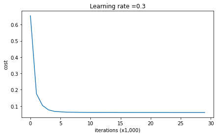
On the train set:
Accuracy: 0.9289099526066351
On the test set:
Accuracy: 0.95
이번에도 테스트세트 정확도가 증가했다
plt.title("Model with dropout")
axes = plt.gca()
axes.set_xlim([-0.75,0.40])
axes.set_ylim([-0.75,0.65])
plot_decision_boundary(lambda x: predict_dec(parameters, x.T), train_X, train_Y)
과적합도 발생하지 않는다
드롭아웃에 대해 정리하면,
✅ 정규화 기법
✅ 학습 단계에서만 사용하고, 테스트에는 사용하지 않는다
✅ 순전파와 역전파 모두에 적용해야 한다
✅ 학습 시 각 드롭아웃 레이어의 출력(활성화값)을 keep_prob으로 나누어주어야 한다 (출력의 기대값을 그대로 유지하기 위함)
--
결론
3가지 모델의 결과는 다음과 같았다
| model | train accuracy | test accuracy |
| 3-layer NN without regularization | 95% | 91.5% |
| 3-layer NN with L2-regularization | 94% | 93% |
| 3-layer NN with dropout | 93% | 95% |
정규화는 훈련세트 정확도는 떨어트린다. 신경망이 훈련세트에 과적합되는것을 막기 때문이다. 그러나 정규화는 테스트세트 정확도를 올리고, 궁극적으로 더 좋은 신경망을 만들어준다.
✅정규화는 과적합을 줄인다
✅정규화는 가중치 값을 낮춘다
✅L2 정규화와 드롭아웃은 효과적인 정규화 기법들이다
