C2W1A3 Gradient Checking
역전파 구현의 정확성을 확인하기 위해 경사 검사를 구현해보자
준비
import numpy as np
from testCases import *
from public_tests import *
from gc_utils import sigmoid, relu, dictionary_to_vector, vector_to_dictionary, gradients_to_vector

%load_ext autoreload
%autoreload 2
미분의 정의는 다음과 같다.
1-Dimensional Gradient Checking
다음은 1차원 선형 모델의 동작이다.
먼저 1차원 선형모델에서 비용함수 J와 그 미분값을 구하기 위한 코드를 구현하고, 경사검사를 사용해 미분 계산이 잘 되었는지 확인해보자
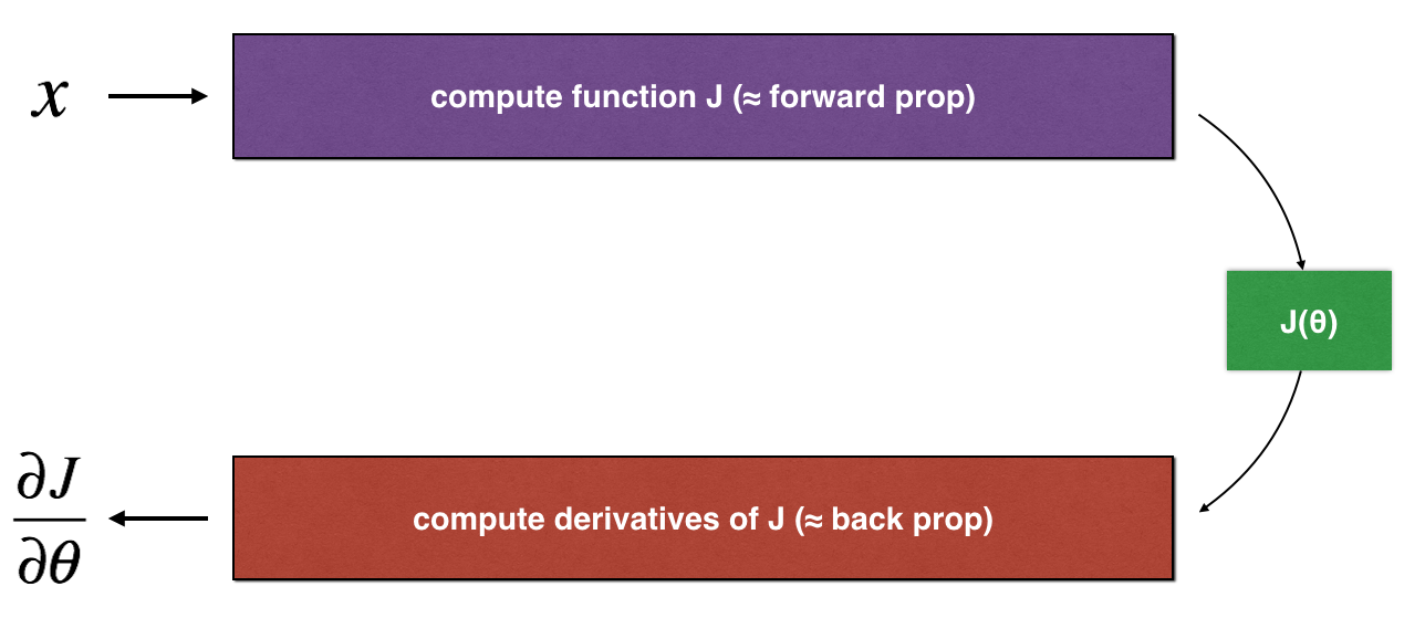
Forward Propagation
순전파에서 비용함수 J를 계산한다.
def forward_propagation(x, theta):
    """
    Implement the linear forward propagation (compute J) presented in Figure 1 (J(theta) = theta * x)

    Arguments:
    x -- a real-valued input
    theta -- our parameter, a real number as well

    Returns:
    J -- the value of function J, computed using the formula J(theta) = theta * x
    """

    J = theta * x

    return J
Backward Propagation
역전파에서 J의 미분값을 계산한다.
def backward_propagation(x, theta):
    """
    Computes the derivative of J with respect to theta (see Figure 1).

    Arguments:
    x -- a real-valued input
    theta -- our parameter, a real number as well

    Returns:
    dtheta -- the gradient of the cost with respect to theta
    """

    dtheta = x

    return dtheta
Gradient Checking
BP에서 dtheta를 잘 계산했는지 확인해보자
-
다음 식들을 활용해 gradapprox를 계산한다
-
BP로 기울기를 계산하고 변수 grad에 저장한다
-
다음 식을 사용하여 gradapprox와 grad 사이의 상대적 차이를 구한다.
차이가 이하라면, 역전파 구현이 잘 되었다고 볼 수 있다
def gradient_check(x, theta, epsilon=1e-7, print_msg=False):
    """
    Implement the gradient checking presented in Figure 1.

    Arguments:
    x -- a float input
    theta -- our parameter, a float as well
    epsilon -- tiny shift to the input to compute approximated gradient with formula(1)

    Returns:
    difference -- difference (2) between the approximated gradient and the backward propagation gradient. Float output
    """

    # Compute gradapprox using right side of formula (1). epsilon is small enough, you don't need to worry about the limit.
    theta_plus = theta + epsilon # Step 1
    theta_minus = theta - epsilon # Step 2
    J_plus = forward_propagation(x, theta_plus) # Step 3
    J_minus = forward_propagation(x, theta_minus) # Step 4
    gradapprox = (J_plus - J_minus) / (2*epsilon) # Step 5

    # Check if gradapprox is close enough to the output of backward_propagation()
    grad = backward_propagation(x, theta)

    numerator = np.linalg.norm(grad-gradapprox) # Step 1'
    denominator = np.linalg.norm(grad) + np.linalg.norm(gradapprox) # Step 2'
    difference = numerator / denominator # Step 3'

    if print_msg:
        if difference > 2e-7:
            print ("\033[93m" + "There is a mistake in the backward propagation! difference = " + str(difference) + "\033[0m")
        else:
            print ("\033[92m" + "Your backward propagation works perfectly fine! difference = " + str(difference) + "\033[0m")

    return difference
아래 코드블럭을 실행시키고 출력 결과를 보면 역전파가 잘 되었는지 확인할 수 있다. difference가 보다 낮으면 잘 되었다고 본다
x, theta = 3, 4
difference = gradient_check(x, theta, print_msg=True)
출력
Your backward propagation works perfectly fine! difference = 7.814075313343006e-11N-dimentional Gradient Checking
이제 n차원 모델에서 경사 검사를 구현해보자
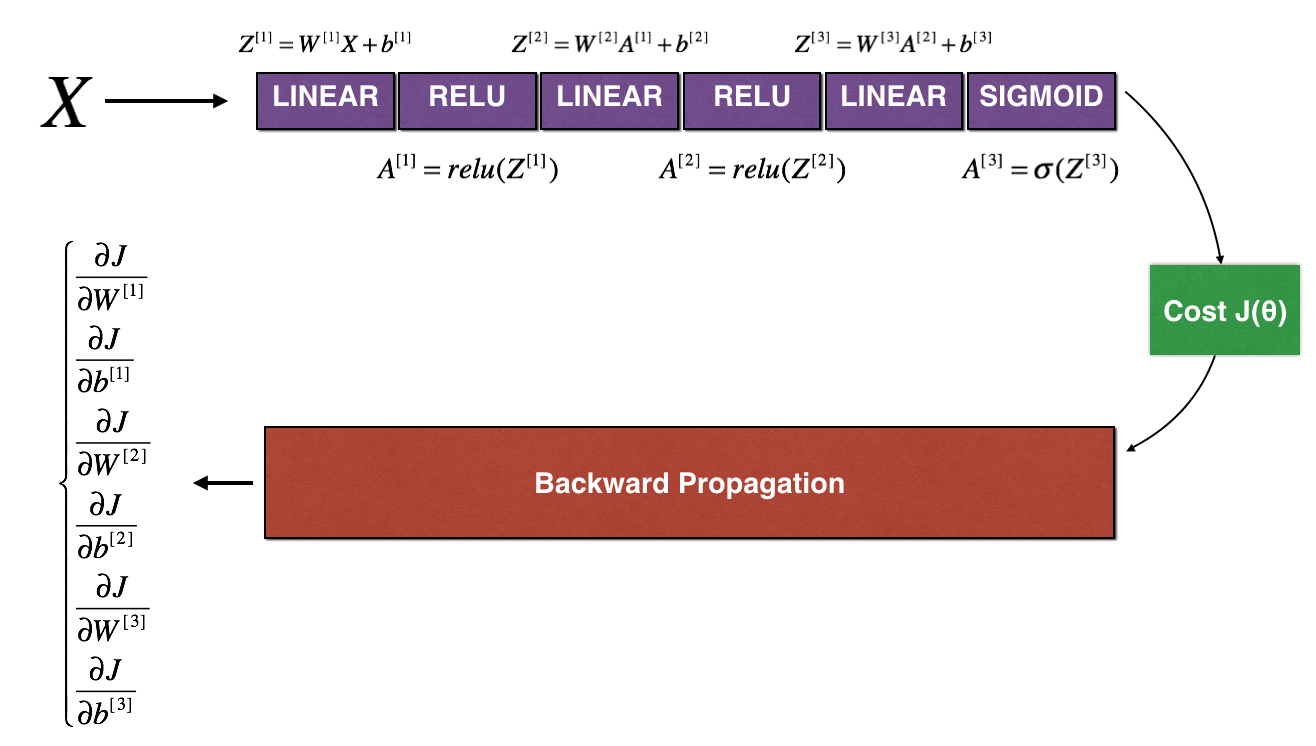
Forward Propagation
def forward_propagation_n(X, Y, parameters):
    """
    Implements the forward propagation (and computes the cost) presented in Figure 3.

    Arguments:
    X -- training set for m examples
    Y -- labels for m examples
    parameters -- python dictionary containing your parameters "W1", "b1", "W2", "b2", "W3", "b3":
                    W1 -- weight matrix of shape (5, 4)
                    b1 -- bias vector of shape (5, 1)
                    W2 -- weight matrix of shape (3, 5)
                    b2 -- bias vector of shape (3, 1)
                    W3 -- weight matrix of shape (1, 3)
                    b3 -- bias vector of shape (1, 1)

    Returns:
    cost -- the cost function (logistic cost for m examples)
    cache -- a tuple with the intermediate values (Z1, A1, W1, b1, Z2, A2, W2, b2, Z3, A3, W3, b3)

    """

    # retrieve parameters
    m = X.shape[1]
    W1 = parameters["W1"]
    b1 = parameters["b1"]
    W2 = parameters["W2"]
    b2 = parameters["b2"]
    W3 = parameters["W3"]
    b3 = parameters["b3"]

    # LINEAR -> RELU -> LINEAR -> RELU -> LINEAR -> SIGMOID
    Z1 = np.dot(W1, X) + b1
    A1 = relu(Z1)
    Z2 = np.dot(W2, A1) + b2
    A2 = relu(Z2)
    Z3 = np.dot(W3, A2) + b3
    A3 = sigmoid(Z3)

    # Cost
    log_probs = np.multiply(-np.log(A3),Y) + np.multiply(-np.log(1 - A3), 1 - Y)
    cost = 1. / m * np.sum(log_probs)

    cache = (Z1, A1, W1, b1, Z2, A2, W2, b2, Z3, A3, W3, b3)

    return cost, cache
Backward Propagation
잘못된 역전파 구현이다. (dW2, db1)
def backward_propagation_n(X, Y, cache):
    """
    Implement the backward propagation presented in figure 2.

    Arguments:
    X -- input datapoint, of shape (input size, 1)
    Y -- true "label"
    cache -- cache output from forward_propagation_n()

    Returns:
    gradients -- A dictionary with the gradients of the cost with respect to each parameter, activation and pre-activation variables.
    """

    m = X.shape[1]
    (Z1, A1, W1, b1, Z2, A2, W2, b2, Z3, A3, W3, b3) = cache

    dZ3 = A3 - Y
    dW3 = 1. / m * np.dot(dZ3, A2.T)
    db3 = 1. / m * np.sum(dZ3, axis=1, keepdims=True)

    dA2 = np.dot(W3.T, dZ3)
    dZ2 = np.multiply(dA2, np.int64(A2 > 0))
    dW2 = 1. / m * np.dot(dZ2, A1.T) * 2
    #dW2 = 1. / m * np.dot(dZ2, A1.T) * 1 # 올바른 구현
    db2 = 1. / m * np.sum(dZ2, axis=1, keepdims=True)

    dA1 = np.dot(W2.T, dZ2)
    dZ1 = np.multiply(dA1, np.int64(A1 > 0))
    dW1 = 1. / m * np.dot(dZ1, X.T)
    db1 = 4. / m * np.sum(dZ1, axis=1, keepdims=True)
    #db1 = 1. / m * np.sum(dZ1, axis=1, keepdims=True) # 올바른 구현

    gradients = {"dZ3": dZ3, "dW3": dW3, "db3": db3,
                 "dA2": dA2, "dZ2": dZ2, "dW2": dW2, "db2": db2,
                 "dA1": dA1, "dZ1": dZ1, "dW1": dW1, "db1": db1}

    return gradients
Gradient Checking
1차원 모델에서 했던것처럼, 역전파에서 계산한 기울기를 gradapprox와 비교한다.
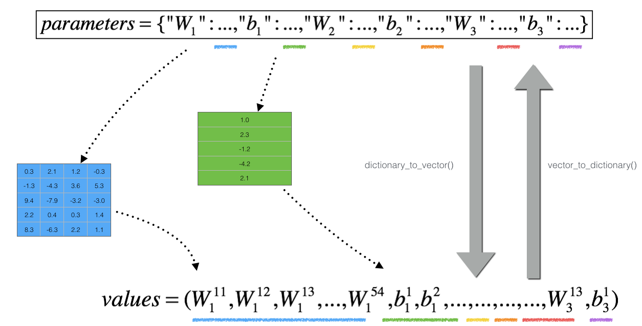
이번에는 가 스칼라가 아니라 딕셔너리(parameters)라는 점이 다르다
딕셔너리 parameters를 벡터 values로, 딕셔너리 gradients를 벡터 grad로 바꾼다. (dictionary_to_vector 함수와 gradients_to_vector 함수는 이미 정의되어 있다)
파라미터 값들을 벡터로 변환하고, 다음 과정을 num_parameters번 반복한다.
J_plus[i]계산
- Set to
np.copy(parameters_values)- Set to
- Calculate using to
forward_propagation_n(x, y, vector_to_dictionary())
-
J_minus[i]계산
대신 를 사용한다 -
계산
벡터 gradapprox의 i번째 원소인
gradapprox[i]는 parameters_values[i]에 대한 기울기의 근사치이다.
다음을 계산해 벡터 gradapprox를 역전파에서 얻은 기울기 벡터와 비교한다.
# GRADED FUNCTION: gradient_check_n

def gradient_check_n(parameters, gradients, X, Y, epsilon=1e-7, print_msg=False):
    """
    Checks if backward_propagation_n computes correctly the gradient of the cost output by forward_propagation_n

    Arguments:
    parameters -- python dictionary containing your parameters "W1", "b1", "W2", "b2", "W3", "b3"
    grad -- output of backward_propagation_n, contains gradients of the cost with respect to the parameters
    X -- input datapoint, of shape (input size, number of examples)
    Y -- true "label"
    epsilon -- tiny shift to the input to compute approximated gradient with formula(1)

    Returns:
    difference -- difference (2) between the approximated gradient and the backward propagation gradient
    """

    # Set-up variables
    parameters_values, _ = dictionary_to_vector(parameters)

    grad = gradients_to_vector(gradients)
    num_parameters = parameters_values.shape[0]
    J_plus = np.zeros((num_parameters, 1))
    J_minus = np.zeros((num_parameters, 1))
    gradapprox = np.zeros((num_parameters, 1))

    # Compute gradapprox
    for i in range(num_parameters):

        # Compute J_plus[i]. Inputs: "parameters_values, epsilon". Output = "J_plus[i]".
        # "_" is used because the function you have outputs two parameters but we only care about the first one
        theta_plus = np.copy(parameters_values) # Step 1
        theta_plus[i][0] = theta_plus[i][0] + epsilon # Step 2
        J_plus[i], _ = forward_propagation_n(X, Y, vector_to_dictionary(theta_plus)) # Step 3

        # Compute J_minus[i]. Inputs: "parameters_values, epsilon". Output = "J_minus[i]".
        theta_minus = np.copy(parameters_values) # Step 1
        theta_minus[i][0] = theta_minus[i][0] - epsilon # Step 2
        J_minus[i], _ = forward_propagation_n(X, Y, vector_to_dictionary(theta_minus)) # Step 3

        # Compute gradapprox[i]
        gradapprox[i] = (J_plus[i] - J_minus[i]) / (2*epsilon)

    # Compare gradapprox to backward propagation gradients by computing difference.
    numerator = np.linalg.norm(grad - gradapprox)
    denominator = np.linalg.norm(grad) + np.linalg.norm(gradapprox)
    difference = numerator / denominator

    if print_msg:
        if difference > 2e-7:
            print ("\033[93m" + "There is a mistake in the backward propagation! difference = " + str(difference) + "\033[0m")
        else:
            print ("\033[92m" + "Your backward propagation works perfectly fine! difference = " + str(difference) + "\033[0m")

    return difference
아래 코드블럭을 실행하면
X, Y, parameters = gradient_check_n_test_case()

cost, cache = forward_propagation_n(X, Y, parameters)
gradients = backward_propagation_n(X, Y, cache)
difference = gradient_check_n(parameters, gradients, X, Y, 1e-7, True)
expected_values = [0.2850931567761623, 1.1890913024229996e-07]
assert not(type(difference) == np.ndarray), "You are not using np.linalg.norm for numerator or denominator"
assert np.any(np.isclose(difference, expected_values)), "Wrong value. It is not one of the expected values"
아래와 같이 출력된다.
| There is a mistake in the backward propagation! | difference = 0.2850931567761623 |
backward_propagation_n 함수로 돌아가, dW2와 db1을 알맞게 고쳐주고 나면
다음과 같은 결과를 얻을 수 있다.
| Your backward propagation works perfectly fine! | difference = 1.1890913024229996e-07 |
- 참고
- 경사 검사는 계산 비용이 많이 들어 느리다. 따라서 매 반복마다 경사검사를 하는 것이 아니라, 기울기가 알맞은지 확인하기 위해 몇 번만 실행한다.
- 드롭아웃을 사용하는 경우에는 경사검사를 사용할 수 없다. 드롭아웃을 끄고 역전파가 올바르게 작동하는지 확인한 후에 드롭아웃을 켜도록 하자
✅ 경사검사는 역전파를 통해 얻은 기울기와 수치적 근사 기울기가 얼마나 근접한지 확인한다.
✅ 경사검사는 느리므로 매 반복마다 실행하지 않는 것이 좋다. 코드가 올바른지 확인하기 위해 몇 번만 실행한 다음, 실제 학습에서는 경사검사 없이 역전파를 사용한다.
이 오타를 한참 못찾았다...