로지스틱 회귀(Logistic Regression)

시험 점수가 합격인지 불합격인인지 정상 메일인지 스팸 메일인지를 분류하는 등
둘 중 하나를 결정하는 문제를 이진 분류(Binary Classification)라고 한다.
그리고 이진 분류를 풀기 위한 대표적인 알고리즘으로 로지스틱 회귀(Logistic Regression)가 있다.

이진 분류(Binary Classification)

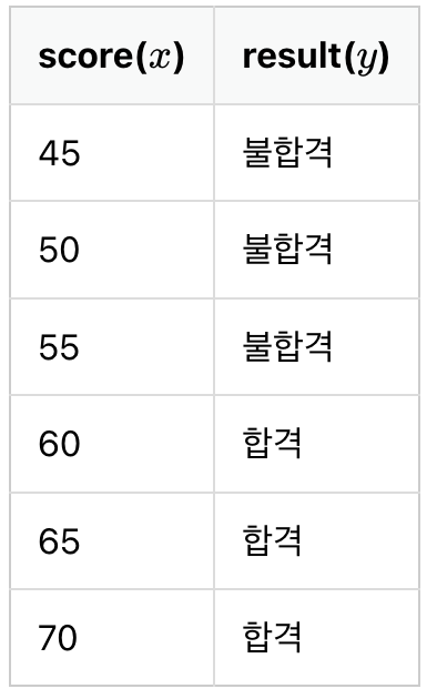
위의 데이터에서 합격을 1, 불합격을 0이라고 하였을 때 그래프를 그려보면 아래와 같다.

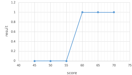
이러한 점들을 표현하는 그래프는 알파벳의 S자 형태로 표현되고, 선형 회귀 때의 직선함수를 통해서 분류하기는 어렵다.
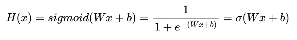
그래서 로지스틱 회귀의 가설은 위의 S자 모양의 그래프를 만들 수 있는 다음과 같은 함수를 사용한다.

시그모이드 함수(Sigmoid function)

로지스틱회귀 역시 선형회귀와 마찬가지로 최적의 W,b를 찾는 것을 목표로 한다.

이 시그모이드 함수에서 W,b가 그래프에 어떤 영향을 주는지 보자.

%matplotlib inline
import numpy as np # 넘파이 사용
import matplotlib.pyplot as plt # 맷플롯립사용

def sigmoid(x): # 시그모이드 함수 정의
    return 1/(1+np.exp(-x))

W = 1, b = 0인 그래프를 보자.

x = np.arange(-5.0, 5.0, 0.1)
y = sigmoid(x)

plt.plot(x, y, 'g')
plt.plot([0,0],[1.0,0.0], ':') # 가운데 점선 추가
plt.title('Sigmoid Function')
plt.show()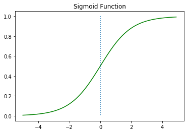

이 때 출력값은 0과 1 사이의 값이고
x = 0일 때 0.5의 값을 가지며

x이 커질 때 1에 수렴, x이 작아질 때 0에 수렴함을 알 수 있다.

이제 W값의 변화에 따른 경사도의 변화를 보자.

x = np.arange(-5.0, 5.0, 0.1)
y1 = sigmoid(0.5*x)
y2 = sigmoid(x)
y3 = sigmoid(2*x)

plt.plot(x, y1, 'r', linestyle='--') # W의 값이 0.5일때
plt.plot(x, y2, 'g') # W의 값이 1일때
plt.plot(x, y3, 'b', linestyle='--') # W의 값이 2일때
plt.plot([0,0],[1.0,0.0], ':') # 가운데 점선 추가
plt.title('Sigmoid Function')
plt.show()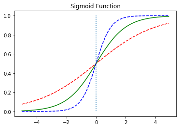

w = 0.5일 때 빨간색 선
w = 1일 때 초록랙 선
w = 2일 때 파란색 선이다.

선형회귀에서 w는 직선의 기울기를 의미했지만 여기서는 그래프의 경사도를 의미한다.
w의 값이 커지면 경사도가 커지고 작아지면 경사도도 작아진다.

이번엔 b값의 변화에 따라 그래프가 어떻게 변하는지 보자.

x = np.arange(-5.0, 5.0, 0.1)
y1 = sigmoid(x+0.5)
y2 = sigmoid(x+1)
y3 = sigmoid(x+1.5)

plt.plot(x, y1, 'r', linestyle='--') # x + 0.5
plt.plot(x, y2, 'g') # x + 1
plt.plot(x, y3, 'b', linestyle='--') # x + 1.5
plt.plot([0,0],[1.0,0.0], ':') # 가운데 점선 추가
plt.title('Sigmoid Function')
plt.show()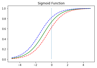

b의 값에 따라 그래프가 좌우로 이동하는 것을 볼 수 있다.

즉 시그모이드 함수의 출력값은 0과 1 사이의 값을 가지는데 이 특성을 이용하여 분류할 수 있다. 예를 들어 임계값을 기준으로 출력값이 임계값 이상이면 1(True), 이하면 0(False)으로 판단하도록 할 수 있다.

비용 함수(Cost function)

로지스틱 회귀의 가설이 H(x) = sigmoid(Wx + b)인 것을 알았다.
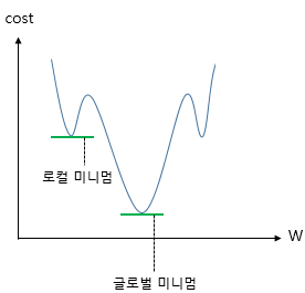
그렇다면 최적의 W,b를 찾기 위한 비용함수는 선형회귀와 같은 평균제곱오차(MSE)를 사용하면 될까?

이 시그모이드 함수를 미분하면 선형회귀때와 달리 non-convex 형태의 그래프가 나온다.

위에서 시그모이드 함수의 특징을 봤는데,
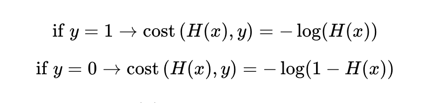
만약 실제값이 1일 때 예측값이 0에 가까워지면 오차가 커져야 하며,
실제값이 0일 때, 예측값이 1에 가까워지면 오차가 커져야 한다.

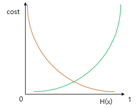
그리고 이를 충족하는 함수가 바로 로그 함수이다.
실제값이 1일 때의 그래프를 주황색 선으로, 실제값이 0일 때의 그래프를 초록색 선으로 표현했다. 이 때 예측값 H(x)이 1이면 오차가 0이므로 cost는 0, H(x)이 0이면 cost는 무한대로 발산한다.

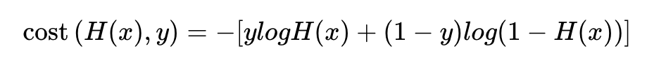
이 로그함수를 식으로 표현하면 다음과 같고

이와 같이 하나의 식으로 표현할 수 있다.

또 선형회귀와 마찬가지로 평균 제곱 오차를 사용하여

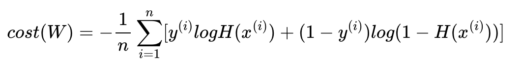
실제값 y와 예측값 H(x)의 차이가 커지면 cost도 커지고
실제값 y와 예측값 H(x)의 차이가 작아지면 cost도 작아진다.

파이토치로 로지스틱 회귀 구현하기

x_data = [[1, 2], [2, 3], [3, 1], [4, 3], [5, 3], [6, 2]]
y_data = [[0], [0], [0], [1], [1], [1]]
x_train = torch.FloatTensor(x_data)
y_train = torch.FloatTensor(y_data)

x_train은 6 × 2의 크기(shape)를 가지는 행렬이며,
y_train은 6 × 1의 크기를 가지는 벡터이다.
x_train을 X, 여기에 곱해지는 가중치 벡터를 W라고 했을 때 W는 2 × 1 이어야 한다.

W = torch.zeros((2, 1), requires_grad=True) # 크기는 2 x 1
b = torch.zeros(1, requires_grad=True)

이 때 가설식은 다음과 같다.

hypothesis = 1 / (1 + torch.exp(-(x_train.matmul(W) + b)))

또는

hypothesis = torch.sigmoid(x_train.matmul(W) + b)

W와 b는 torch.zeros를 통해 전부 0으로 초기화 된 상태로,
예측값은 실제값 y_train과 크기가 동일한 6 × 1의 크기를 가지는 0.5 벡터가 나온다.

print(hypothesis) # 예측값인 H(x) 출력

tensor([[0.5000],
        [0.5000],
        [0.5000],
        [0.5000],
        [0.5000],
        [0.5000]], grad_fn=<MulBackward>)

이제 비용함수(예측값과 실제값 사이 cost)를 구해보자.

print(hypothesis)
print(y_train)

tensor([[0.5000],
        [0.5000],
        [0.5000],
        [0.5000],
        [0.5000],
        [0.5000]], grad_fn=<SigmoidBackward>)
tensor([[0.],
        [0.],
        [0.],
        [1.],
        [1.],
        [1.]])

이 때 하나의 샘플에 대해서만 오차를 구해보자.

-(y_train[0] * torch.log(hypothesis[0]) + 
  (1 - y_train[0]) * torch.log(1 - hypothesis[0]))

tensor([0.6931], grad_fn=<NegBackward>)

이제 모든 원소에 대해 오차를 구해보자.

losses = -(y_train * torch.log(hypothesis) + 
           (1 - y_train) * torch.log(1 - hypothesis))
print(losses)

tensor([[0.6931],
        [0.6931],
        [0.6931],
        [0.6931],
        [0.6931],
        [0.6931]], grad_fn=<NegBackward>)

그리고 이 전체 오차에 대한 평균을 구하면

cost = losses.mean()
print(cost)

tensor(0.6931, grad_fn=<MeanBackward1>)

cost는 0.6931이다.

그런데 위에서 긴 수식으로 귀찮게 적었는데 사실 파이토치에서

torch.nn.functional as F
F.binary_cross_entropy(예측값, 실제값)

으로 비용함수를 사용할 수 있다. 껄껄. 즉

F.binary_cross_entropy(hypothesis, y_train) #tensor(0.6931, grad_fn=<BinaryCrossEntropyBackward0>)

그럼 모델 훈련까지 시켜보자.

x_data = [[1, 2], [2, 3], [3, 1], [4, 3], [5, 3], [6, 2]]
y_data = [[0], [0], [0], [1], [1], [1]]
x_train = torch.FloatTensor(x_data)
y_train = torch.FloatTensor(y_data)

# 모델 초기화
W = torch.zeros((2, 1), requires_grad=True)
b = torch.zeros(1, requires_grad=True)
# optimizer 설정
optimizer = optim.SGD([W, b], lr=1)

nb_epochs = 1000
for epoch in range(nb_epochs + 1):

    # Cost 계산
    hypothesis = torch.sigmoid(x_train.matmul(W) + b)
    cost = -(y_train * torch.log(hypothesis) + 
             (1 - y_train) * torch.log(1 - hypothesis)).mean()

    # cost로 H(x) 개선
    optimizer.zero_grad()
    cost.backward()
    optimizer.step()

    # 100번마다 로그 출력
    if epoch % 100 == 0:
        print('Epoch {:4d}/{} Cost: {:.6f}'.format(
            epoch, nb_epochs, cost.item()
        ))

이제 W와 b를 가지고 예측값을 출력해보자.

hypothesis = torch.sigmoid(x_train.matmul(W) + b)
print(hypothesis)

hypothesis = torch.sigmoid(x_train.matmul(W) + b)
print(hypothesis)

모두 0과 1 사이의 값을 가지고 있다.
이제 0.5를 넘으면 True, 넘지 않으면 False로 값을 정하여 출력해보자.

prediction = hypothesis >= torch.FloatTensor([0.5])
print(prediction)

tensor([[False],
        [False],
        [False],
        [ True],
        [ True],
        [ True]])

훈련이 된 후의 W와 b의 값을 출력해보자.

print(W)
print(b)

tensor([[3.2530],
        [1.5179]], requires_grad=True)
tensor([-14.4819], requires_grad=True)

nn.Module로 구현하는 로지스틱 회귀

선형회귀의 가설식을 구현하기 위해서는 nn.Linear()를 사용했었다.
파이토치에서는 nn.Sigmoid()를 통해서 시그모이드 함수를 구현한다.

nn.Linear()의 결과를 nn.Sigmoid()를 거치게하면 로지스틱 회귀의 가설식이 된다.

파이토치의 nn.Linear와 nn.Sigmoid로 로지스틱 회귀 구현하기

x_data = [[1, 2], [2, 3], [3, 1], [4, 3], [5, 3], [6, 2]]
y_data = [[0], [0], [0], [1], [1], [1]]
x_train = torch.FloatTensor(x_data)
y_train = torch.FloatTensor(y_data)

nn.Sequential()은 nn.Module 층을 차례로 쌓을 수 있도록 한다. 즉 여러 함수들을 연결해주는 역할을 한다.

model = nn.Sequential(
   nn.Linear(2, 1), # input_dim = 2, output_dim = 1
   nn.Sigmoid() # 출력은 시그모이드 함수를 거친다
)

W와 b는 랜덤 초기화가 된 상태인데 훈련 데이터를 넣어 예측값을 확인해보자.

model(x_train)

6 × 1 크기의 예측값 텐서가 출력된다.경사 하강법을 사용하여 훈련해보자.

# optimizer 설정
optimizer = optim.SGD(model.parameters(), lr=1)

nb_epochs = 1000
for epoch in range(nb_epochs + 1):

    # H(x) 계산
    hypothesis = model(x_train)

    # cost 계산
    cost = F.binary_cross_entropy(hypothesis, y_train)

    # cost로 H(x) 개선
    optimizer.zero_grad()
    cost.backward()
    optimizer.step()

    # 20번마다 로그 출력
    if epoch % 10 == 0:
        prediction = hypothesis >= torch.FloatTensor([0.5]) # 예측값이 0.5를 넘으면 True로 간주
        correct_prediction = prediction.float() == y_train # 실제값과 일치하는 경우만 True로 간주
        accuracy = correct_prediction.sum().item() / len(correct_prediction) # 정확도를 계산
        print('Epoch {:4d}/{} Cost: {:.6f} Accuracy {:2.2f}%'.format( # 각 에포크마다 정확도를 출력
            epoch, nb_epochs, cost.item(), accuracy * 100,
        ))

실행해보면 중간부터 정확도가 100%이 나온다.기존의 훈련 데이터를 입력하여 예측값을 확인해보자.

model(x_train)

tensor([[2.7943e-04],
        [3.1737e-02],
        [3.9147e-02],
        [9.5604e-01],
        [9.9822e-01],
        [9.9968e-01]], grad_fn=<SigmoidBackward0>)

훈련 후의 W와 b의 값을 출력해보자.

print(list(model.parameters()))

[Parameter containing:
tensor([[3.2488, 1.5156]], requires_grad=True), Parameter containing:
tensor([-14.4626], requires_grad=True)]

굿굿..

인공 신경망으로 표현되는 로지스틱 회귀

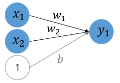
위의 그림은 인공 신경망이다.
이 그림에서 각 화살표는 입력과 곱해지는 가중치 또는 편향입니다.
각 입력에 대해서 검은색 화살표는 가중치, 회색 화살표는 편향이 곱해진다.
각 입력 x는 각 입력의 가중치 w와 곱해지고, 편향 b는 상수 1과 곱해지는 것으로 표현했고
출력하기 전에 시그모이드 함수를 지나게 된다.

즉 위 그림은 다음과 같은 다중 로지스틱 회귀를 표현한다.

H(x) = sigmoid(x1w1 + x2w2 + b)

클래스로 파이토치 모델 구현하기

x_data = [[1, 2], [2, 3], [3, 1], [4, 3], [5, 3], [6, 2]]
y_data = [[0], [0], [0], [1], [1], [1]]
x_train = torch.FloatTensor(x_data)
y_train = torch.FloatTensor(y_data)

class BinaryClassifier(nn.Module):
    def __init__(self):
        super().__init__()
        self.linear = nn.Linear(2, 1)
        self.sigmoid = nn.Sigmoid()

    def forward(self, x):
        return self.sigmoid(self.linear(x))

model = BinaryClassifier()

# optimizer 설정
optimizer = optim.SGD(model.parameters(), lr=1)

nb_epochs = 1000
for epoch in range(nb_epochs + 1):

    # H(x) 계산
    hypothesis = model(x_train)

    # cost 계산
    cost = F.binary_cross_entropy(hypothesis, y_train)

    # cost로 H(x) 개선
    optimizer.zero_grad()
    cost.backward()
    optimizer.step()

    # 20번마다 로그 출력
    if epoch % 10 == 0:
        prediction = hypothesis >= torch.FloatTensor([0.5]) # 예측값이 0.5를 넘으면 True로 간주
        correct_prediction = prediction.float() == y_train # 실제값과 일치하는 경우만 True로 간주
        accuracy = correct_prediction.sum().item() / len(correct_prediction) # 정확도를 계산
        print('Epoch {:4d}/{} Cost: {:.6f} Accuracy {:2.2f}%'.format( # 각 에포크마다 정확도를 출력
            epoch, nb_epochs, cost.item(), accuracy * 100,
        ))