1. Welcome

2. Pre-Notebook

3. Notbook Workspace

4. Single layer neural networks

파이토치를 활용한 간단한 neural network 만들기

• 순서

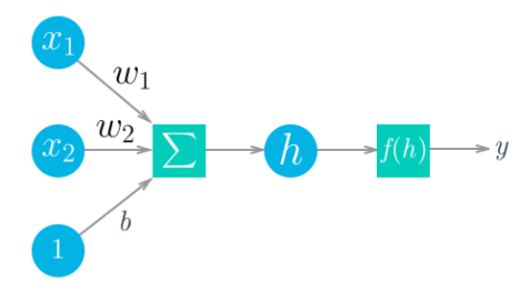
1. 입력값에 가중치를 곱해 합한 다음 h를 구한다.
2. 함수에 h 값을 삽입하여 결과 값 y를 구해낸다.
3. 위의 과정의 반복

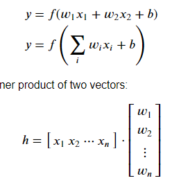
위를 수식으로 표현하면 위와 같은 식으로 만들 수 있다.

이때 데이터 배열과 그 모음을 텐서라고 부른다.

# 라이브러리
import pytorch

# fake data 생성
torch.manual_seed(7) # 랜덤 함수에서 사용하는 랜덤 시드값

# [1 row, 5 columns]의 랜덤값을 가진 행열 텐서
features = torch.randn((1, 5))
# features와 
weights = torch.randn_like(features)
# and a true bias term
bias = torch.randn((1, 1))
features, weights, bias

5. Single layer neural networks solution

6. Networks Using Matrix Multiplication

7. Multilayer Networks Solution

8. Neural Networks in PyTorch

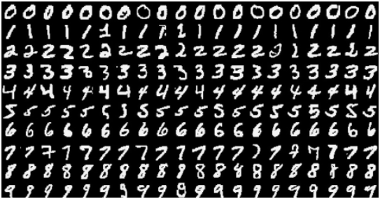
MNIST는 흑백의 손글씨 숫자들이다.
28 x 28

목표 : 이미지의 정확한 번호가 무엇인지 확인하기

# Import necessary packages

%matplotlib inline #jupyter notebook 에 그래프를 그리어 주는 기능
%config InlineBackend.figure_format = 'retina'

import numpy as np
import torch

import helper

import matplotlib.pyplot as plt

### Run this cell

from torchvision import datasets, transforms

# Define a transform to normalize the data
transform = transforms.Compose([transforms.ToTensor(),
                              transforms.Normalize((0.5,), (0.5,)),
                              ])

# Download and load the training data
trainset = datasets.MNIST('~/.pytorch/MNIST_data/', download=True, train=True, transform=transform)
trainloader = torch.utils.data.DataLoader(trainset, batch_size=64, shuffle=True)

그래서 pytorch 로 부터 MNIST 데이타를 받아오고 trainloader 에 데이터를 저장한다.
이때 우리는 batch_size를 64로 맞추어 두었기 때문에 이미지를 받을 때마다 64개의 이미지를 받게 된다.

for image, label in trainloader:

앞으로는 반복문을 이용하여서 image 와 label을 받을 수 있다.

dataiter = iter(trainloader)
images, labels = dataiter.next()
print(type(images))
print(images.shape)
print(labels.shape)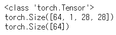

이때 images.shape를 활용하여 출력 결과를 보면
64는 64개의 이미지 / 1은 color 채널(0과 1의 흑과 백만 존재한다) / 28, 28은 이미지의 행과 열 비트를 의미한다.

plt.imshow(images[1].numpy().squeeze(), cmap='Greys_r');

받아온 이미지를 실재로 출력해 보면

위와 같은 숫자가 흑백으로 출력된 것을 확인할 수 있다.

9. Neural Networks Solution

이제 이렇게 받아온 이미지들을 활용하여 Neural Network를 제작하여 보자 제작할때는

## 시그모이드 함수를 사용하기로 하였다.
def activation(x):
    return 1/(1+torch.exp(-x))

# images.shape[0] : 이미지의 길이 / -1 : 1번 인자와 비슷하게 값을 입력
inputs = images.view(images.shape[0],-1)

# create parameters
# input : 784 / hidden : 256
w1 = torch.randn(784,256)
b1=torch.randn(256)

#input : 256 / output : 10
w2 = torch.randn(256,10)
b2 = torch.randn(10)

h = activation(torch.mm(inputs,w1)+b1)

# 
out = torch.mm(h,w2)+b2# output of your network, should have shape (64,10)
print(out.shape)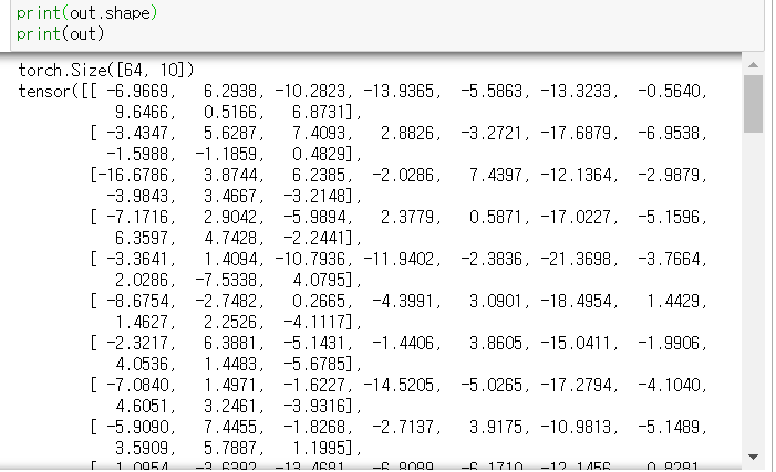

최종결과물은 (64,10) 크기의 데이터들이 나온 것을 확인할 수 있다.

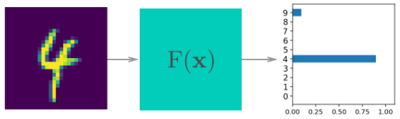
이제 이렇게 나온 값들을 우리가 만든 네트워크에 통과시키어서 우리의 이미지가 과연 어떤 것인지에 대한 가능성도(확률)을 구해낼 수 있다.

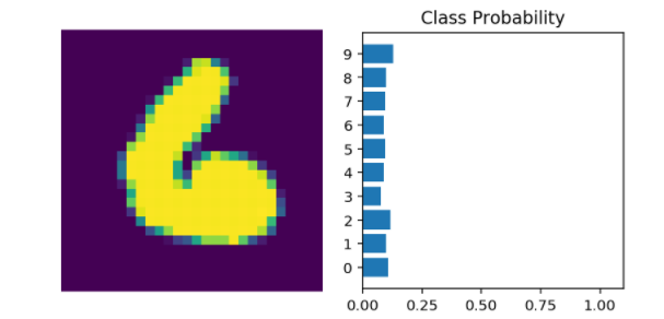
하지만 위의 probability를 보면 대다수가 비슷비슷한 것을 볼 수 있다. 즉 우리의 이미지가 무엇인지 아는 것이 쉽지 않다는 것이다.

이것을 알아볼 수 있도록 만들기 위해 softmax함수를 사요아여야 한다. Softmax(소프트맥스)는 입력받은 값을 출력으로 0~1사이의 값으로 모두 정규화하며 출력 값들의 총합은 항상 1이 되는 특성을 가진 함수이다.

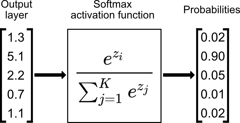
위의 함수를 사용하여서 값을 구해낼 수 있다. 그리고 그 값의 합은 항상 1이 된다.

10. Implementing Softmax Solution

## Solution
# 우리가 구한 out변수는 64, 10 의 변수이기 때문에 sum을 그냥 나누어 줄 수 없다.
# 그래서 view 를 사용하여 64, 1크기로 바꾸어 준다음 모든 항을 나누어 주었다.
def softmax(x):
    return torch.exp(x)/torch.sum(torch.exp(x), dim=1).view(-1, 1)

probabilities = softmax(out)

# Does it have the right shape? Should be (64, 10)
print(probabilities.shape)
# Does it sum to 1?
print(probabilities.sum(dim=1))

---

Building networks with PyTorch

이제 PyTorch를 활용하여서 neural network를 구현하여 보자

from torch import nn

# 사용법은 nn의 Module 클래스를 상속 받아와서 수정하여 사용하면 된다.
class Network(nn.Module):
    def __init__(self):
        super().__init__()
        
        # 출력될 행열의 행과 열을 맞추어 준다.
        # Inputs to hidden layer linear transformation
        self.hidden = nn.Linear(784, 256)
        # Output layer, 10 units - one for each digit
        self.output = nn.Linear(256, 10)
        
        # Define sigmoid activation and softmax output 
        self.sigmoid = nn.Sigmoid()
        self.softmax = nn.Softmax(dim=1)
        
    # 실질적으
    def forward(self, x):
        # Pass the input tensor through each of our operations
        x = self.hidden(x)
        x = self.sigmoid(x)
        x = self.output(x)
        x = self.softmax(x)
        
        return x

pytorch의 nn을 활용하여서 네트워크를 구현하도록 제작하였다. 이러한 방식으로 제작하여야만 더 큰 네트워크도 감당할 수 있게 되기 때문이였다.

# Create the network and look at it's text representation
model = Network()
model

클래스를 보기 위해 객체를 생성하고 이를 호출하면

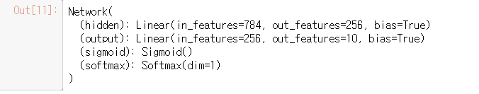
다음과 같이 클래스 내부에 뭐가 있는지 볼 수 있다.

import torch.nn.functional as F

class Network(nn.Module):
    def __init__(self):
        super().__init__()
        # Inputs to hidden layer linear transformation
        self.hidden = nn.Linear(784, 256)
        # Output layer, 10 units - one for each digit
        self.output = nn.Linear(256, 10)
        
    def forward(self, x):
        # Hidden layer with sigmoid activation
        x = F.sigmoid(self.hidden(x))
        # Output layer with softmax activation
        x = F.softmax(self.output(x), dim=1)
        
        return x

좀 더 정밀하게 네트워크를 구성하기 위해 functional을 사용하는 것도 좋은 방법이며 우리는 앞으로 이 라이브러리를 더 많이 사용할 예정이다.

이때 Activation function들도 여러가지로 나뉘게 되는데

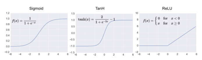
보통은 ReLU를 가장 많이 사용한다.

최종적으로 만들어진 모델은 다음과 같이 수십개의 입력이 h로 들어가서 결과를 반환하는 형태로 만들어 진다.

11. Network Architectures in PyTorch

Training Neural Networks

이제 신경망에 우리의 데이터를 학습시키어야 한다. 기존에 있는 모델은 우리의 입력값에 대해 명확한 해답을 제시해 주지 못하였다. 이제 우리는 함수에 입력을 넣음 다음 어떠한 값인지에 대한 가능성(probability)을 얻어내는 과정을 거치게 될 것이다.

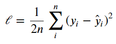
처음으로 우리가 할 것은 loss function이다. 이것은 우리가 얼마나 원하는 결과값으로 부터 멀어졌는지(일치하지 않는지)를 알아봐 주는 함수이다.

우리가 해야하는 일은 가중치값을 조절하여서 이 loss function의 값을 minimize 해주는 일을 해주어야 한다.

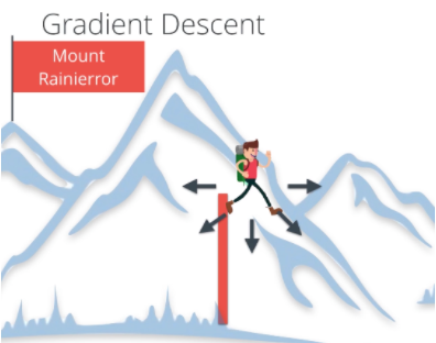
앞으로 우리는 이러한 과정을 Gradient Descent라고 부르도록 하자. 마치 산을 올라가듯이 위로 올라갈 수록 loss function의 값은 작아지고 accuracy를 증가하게 된다.

Backpropagation

만약 단순히 하나의 신경망이면 Gradient Descent의 수행은 매우 단순하다. 하지만 우리가 다루게 될 신경망은 겹겹이 쌓여진 복잡한 신경망이다. 이러한 문제점을 해결하기 위해 Backpropagtaion을 사용한다.

Forward pass를 할 경우 가장 아래에서부터 꼭대기로 점진적으로 움직이는 형태를 띄게 된다.
반대로 Backward pass는 Forward pass를 통해 구해낸 값의 차이를 구한 후 그 오차값을 다시 뒤로 전파해가면서 각 노드가 가지고 있는 변수들을 갱신하는 알고리즘이다.

그럼 어떻게 각 노드가 가지고 있는 weight와 bias 계산할 수 있을까? 또한 Multi Layer Network에서 각 노드나 레이어가 가지고 있는 변수들은 다 제 각각인데 그 값들을 얼마나 변경하는 지 알 수 있을까? 이런 문제를 해결하기 위해 우리는 Chain Rule을 사용하여야 한다.

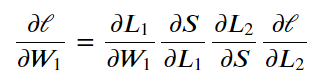
미분이 가능하다 = 기울기를 구한다 라는 것은 변화량을 구한다는 것이다.
1. 그렇기에 Chain Rule이란 쉽게 말해 x가 변화했을 때 함수 g가 얼마나 변화하였는 지
1. 그로 인해 함수 g의 변화로 안해 함수 f가 얼마나 변화하였는지 알 수 있고
1. 함수 f의 인자가 함수 g이면 최종 값 F의 변화량에 기여하는 각 함수 f와 g의 기여도를 알 수 있다.

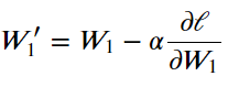
그리고 이때 정확한 변화 값을 알기 위해 사용하는 것이 위의 공식이며 이때 α값이 곧 변화될 가중치 값이다.

Losses in PyTorch

PyTorch에서는 Loss값을 구하는 nn.CrossEntropyLoss를 제공한다.

import torch
from torch import nn
import torch.nn.functional as F
from torchvision import datasets, transforms

# Define a transform to normalize the data
transform = transforms.Compose([transforms.ToTensor(),
                                transforms.Normalize([0.5], [0.5]),
                              ])
# Download and load the training data
trainset = datasets.MNIST('~/.pytorch/MNIST_data/', download=True, train=True, transform=transform)
trainloader = torch.utils.data.DataLoader(trainset, batch_size=64, shuffle=True)

12. Network Architectrues Solution

강의에서는 Softmax를 LogSoftmax로 사용하는 것이 더 좋다고 이야기하며 nn.LogSoftmax를 소개해주었습니다.

LogSoftmax는 Softmax에 비해서 overflow나 underflow가 생길가능성이 낮습니다. 아래는 해당공식들로 Softmax에 Log를 붙여서 출력해줍니다.

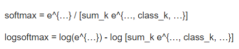
이때 LogSoftmax는 행 또는 열을 기준으로 합칠 수가 있는데 이를 dim이라고 부릅니다. dim=0 이면 행으로 합하고 dim=1 이면 열로 합합니다.

## Solution

# Build a feed-forward network
model = nn.Sequential(nn.Linear(784, 128),
                      nn.ReLU(),
                      nn.Linear(128, 64),
                      nn.ReLU(),
                      nn.Linear(64, 10),
                      nn.LogSoftmax(dim=1))

# Define the loss
criterion = nn.NLLLoss()

# Get our data
images, labels = next(iter(trainloader))
# Flatten images
images = images.view(images.shape[0], -1)

# Forward pass, get our log-probabilities
logps = model(images)
# Calculate the loss with the logps and the labels
loss = criterion(logps, labels)

print(loss)

Autograd

이제 backpropagation을 수행에 있어서 Loss를 이용하여야 한다. 이를 위해 pyTorch 에서는 Autograd 함수를 제공하여 준다.

x = torch.randn(2,2, requires_grad=True)
print(x)

이제 backward을 위해 랜덤한 텐서를 생성하는데 이때 requires_grad를 True로 맞추어 둔다.

이후 텐서가 저장되어 있는 변수 z에 z.backward()를 활용하여서 backward 결과를 얻어낼 수 있다.

x = torch.randn(2,2, requires_grad=True)

y = x**2

z = y.mean()

print(x.grad)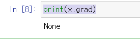

z.backward()
print(x.grad)
print(x/2)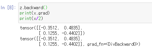

Loss and Autograd together

이제 Loss와 backward를 동시에 수행해 보자

# loss구하기
model = nn.Sequential(nn.Linear(784, 128),
                      nn.ReLU(),
                      nn.Linear(128, 64),
                      nn.ReLU(),
                      nn.Linear(64, 10),
                      nn.LogSoftmax(dim=1))

criterion = nn.NLLLoss()
images, labels = next(iter(trainloader))
images = images.view(images.shape[0], -1)

logps = model(images)
loss = criterion(logps, labels)

# backpropagation
print('Before backward pass: \n', model[0].weight.grad)

loss.backward()

print('After backward pass: \n', model[0].weight.grad)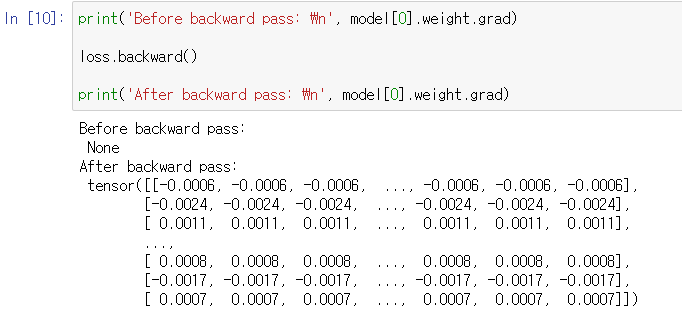

Training the network!

이제 loss와 backward를 할 줄 알았으니 실재 network를 훈련시키어 보자
이를 위해 pyTorch에서는 optim 클래스를 제공하여 준다.

from torch import optim

# Optimizers require the parameters to optimize and a learning rate
optimizer = optim.SGD(model.parameters(), lr=0.01)

순서는 아래와 같다.
1. forward pass 즉 답을 우선 구해낸다.
1. network output으로 loss를 구해낸다.
1. backward를 수행하여서 gradient값을 구해낸다.
1. optimizer로 weight를 새로고침한다.

print('Initial weights - ', model[0].weight)

images, labels = next(iter(trainloader))
images.resize_(64, 784)

# Clear the gradients, do this because gradients are accumulated
optimizer.zero_grad()

# Forward pass, then backward pass, then update weights
output = model(images)
loss = criterion(output, labels)
loss.backward()
print('Gradient -', model[0].weight.grad)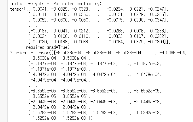

# Take an update step and few the new weights
optimizer.step()
print('Updated weights - ', model[0].weight)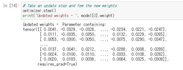

13. Training a Network Solution

실재 데이터를 가지고 loss를 구하여 보면 다음과 같은 결과가 나오게 된다.

model = nn.Sequential(nn.Linear(784, 128),
                      nn.ReLU(),
                      nn.Linear(128, 64),
                      nn.ReLU(),
                      nn.Linear(64, 10),
                      nn.LogSoftmax(dim=1))

criterion = nn.NLLLoss()
optimizer = optim.SGD(model.parameters(), lr=0.003)

epochs = 5
for e in range(epochs):
    running_loss = 0
    for images, labels in trainloader:
        # Flatten MNIST images into a 784 long vector
        images = images.view(images.shape[0], -1)
    
        # TODO: Training pass
        optimizer.zero_grad()
        
        output = model(images)
        loss = criterion(output, labels)
        loss.backward()
        optimizer.step()
        
        running_loss += loss.item()
    else:
        print(f"Training loss: {running_loss/len(trainloader)}")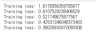

이렇게 학습된 모델은 우리가 넣은 값에서 예측을 할 수 있게 된다.

%matplotlib inline
import helper

images, labels = next(iter(trainloader))

img = images[0].view(1, 784)
# Turn off gradients to speed up this part
with torch.no_grad():
    logps = model(img)

# Output of the network are log-probabilities, need to take exponential for probabilities
ps = torch.exp(logps)
helper.view_classify(img.view(1, 28, 28), ps)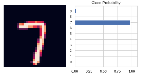

14. Classifying Fashion-MNIST

Classifying Clothing Images

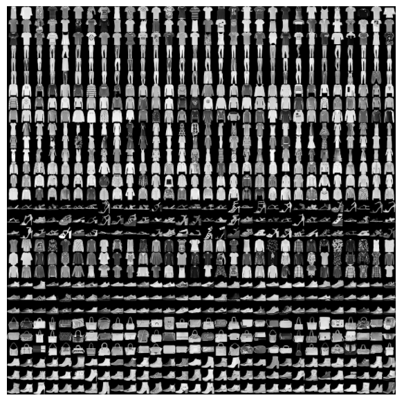
이번에는 MNIST의 datasets.FashionMNIST를 이용하여서 옷에 대한 데이터를 받아오고 예측해 보자

15. Fashion-MNIST Solution

16. Inference and Validation

inference(추론) : 우리가 예측한 모델과 이 모델을 사용하여 데이터를 예측하는 과정
overfitting : 모델이 실제 분포보다 학습 샘플들 분포에 더 근접하게 학습되는 현상 - 모델은 새로운 데이터 보다 기존에 학습된 데이터에 저 근접한 결과를 반환한다. 이러한 문제점을 해결하기 위해 regularization을 수행하여야 한다.
underfitting : 모델이 학습 오류를 줄이지 못하는 상황
validation(검증) : 어떤 데이터 값이 유효하거나 타당한지를 확인하는 것