스터디노트 (Tensorflow 3)

Linear Regression 구현해보기

import tensorflow as tf
import matplotlib.pyplot as plt
import numpy

tf.random.set_seed(777)

가상 데이터셋

W_true = 3.0
B_true = 2.0

X = tf.random.normal((500, 1))
noise = tf.random.normal((500, 1))

y = X * W_true + B_true + noise

plt.scatter(X, y)
plt.show()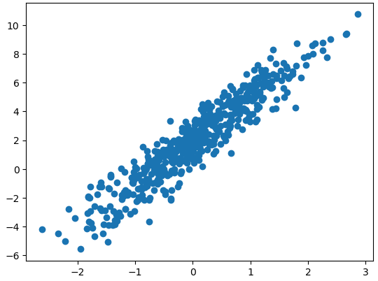

w = tf.Variable(5.)
b = tf.Variable(0.)

lr = 0.03

# 학습 과정 기록
w_records = []
b_recodes = []
loss_records = []

for epoch in range(100):
    # 매 epoch 마다 학습을 할 것이다.
    with tf.GradientTape() as tape:
        y_hat = X * w + b
        loss = tf.reduce_mean(tf.square(y - y_hat))
    w_records.append(w.numpy())
    b_recodes.append(b.numpy())
    dw, db = tape.gradient(loss, [w, b])
    
    loss_records.append(loss.numpy())
    
    w.assign_sub(lr*dw)
    b.assign_sub(lr*db)
    

plt.plot(loss_records)
plt.title('loss')
plt.show()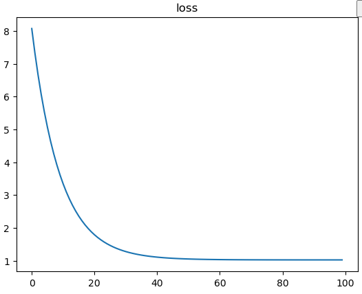

plt.plot(w_records)
plt.title('w')
plt.show()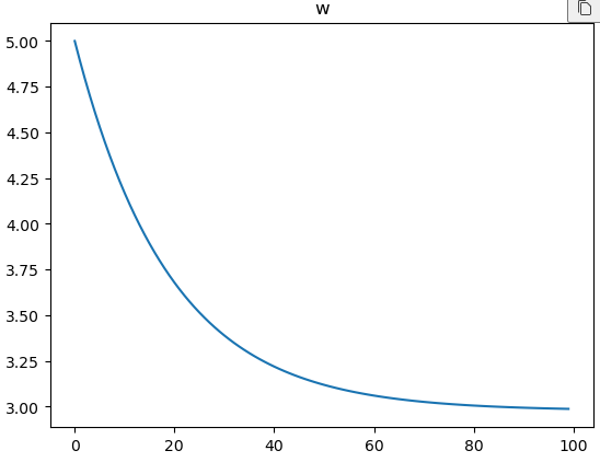

plt.plot(b_recodes)
plt.title('b')
plt.show()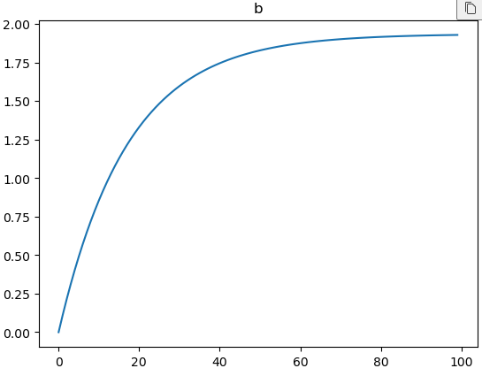

X[0] * w + b

y[0]

Dataset 당뇨병 진행도 예측 하기

from sklearn.datasets import load_diabetes
import pandas as pd
import numpy as np
import tensorflow as tf

diabetes = load_diabetes()
df = pd.DataFrame(diabetes.data, columns=diabetes.feature_names, dtype=np.float32)
df['const'] = np.ones(df.shape[0])
df.tail(3)

$X$ 를 Feature, ,$w$를 가중치 벡터, $y$를 Target이라고 할 때,

$X^T X$의 역행령이 존재 한다고 가정했을 때,

아래의 식을 이용해 $w$의 추정치 $w^*$를 구해봅시다.

X =df
y = np.expand_dims(diabetes.target, axis=1)
# diabetes.target.shape

XT = tf.transpose(X)

w = tf.matmul(tf.matmul(tf.linalg.inv(tf.matmul(XT, X)), XT), y)

y_pred = tf.matmul(X, w)

print('예측한 진행도 : ', y_pred[0].numpy(), '실제 진행도 : ', y[0])
print('예측한 진행도 : ', y_pred[19].numpy(), '실제 진행도 : ', y[19])
print('예측한 진행도 : ', y_pred[31].numpy(), '실제 진행도 : ', y[31])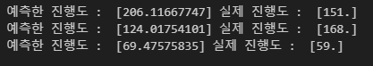

이번에는, SGD 방식으로 구현해보세요!!

• Conditions
  • steepest gradient descents(전체 데이터 사용)
  • 가중치는 Gaussian normal distribution에서의 난수로 초기화함.
  • step size == 0.03
  • 100 iteration

lr = 0.03
num_iter = 100

w_init = tf.random.normal((X.shape[-1], 1), dtype=tf.float64) # X의 feature개수, 1
w = tf.Variable(w_init)

X.dtypes

for i in range(num_iter):
    with tf.GradientTape() as tape:
        y_hat = tf.matmul(X, w)
        loss = tf.reduce_mean((y - y_hat)**2)
    
    dw = tape.gradient(loss, w)
    w.assign_sub(lr * dw)

print('예측한 진행도 : ', y_hat[0].numpy(), '실제 진행도 : ', y[0])
print('예측한 진행도 : ', y_hat[19].numpy(), '실제 진행도 : ', y[19])
print('예측한 진행도 : ', y_hat[31].numpy(), '실제 진행도 : ', y[31])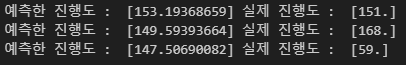

perceptron

import tensorflow as tf
import numpy as np 

이번엔 Iris 데이터 중 두 종류를 분류하는 퍼셉트론을 제작한다. y값은 1 또는 -1을 사용하고 활성화 함수로는 하이퍼탄젠트(hypertangent)함수를 사용한다.

$\Large{ \hat{y} = tanh(w^Tx) }$

비용 함수로는 다음 식을 사용한다.

from sklearn.datasets import load_iris
iris = load_iris()
print(iris.DESCR)

idx = np.in1d(iris.target, [0, 2])
X_data = iris.data[idx, 0:2]
y_data = (iris.target[idx] - 1.0)[:, np.newaxis] 

X_data.shape, y_data.shape

이 데이터를 이용해 Perceptron을 구현해보세요!

• 데이터 하나당 한번씩 weights 업데이트
• step size == 0.0003
• iteration == 200

num_iter = 500
lr = 0.0003

w = tf.Variable(tf.random.normal([2, 1], dtype=tf.float64))
b = tf.Variable(tf.random.normal([1, 1], dtype=tf.float64))

zero = tf.constant(0, dtype=tf.float64)

for epoch in range(num_iter):
    for i in range(X_data.shape[0]):
        x = X_data[i : i+1]
        y = y_data[i : i+1]
        
        with tf.GradientTape() as tape:
            logit = tf.matmul(x, w) + b
            y_hat = tf.tanh(logit) # 예측치
            loss = tf.maximum(zero, tf.multiply(-y, y_hat))
            
        grad = tape.gradient(loss, [w, b])
        
        w.assign_sub(lr * grad[0])
        b.assign_sub(lr * grad[1])
        

y_pred = tf.tanh(tf.matmul(X_data, w) + b)

X_data[0].shape

print('예측치 : ', -1 if y_pred[0] < 0 else 1 , '정답 : ', y_data[0])
print('예측치 : ', -1 if y_pred[51] < 0 else 1 , '정답 : ', y_data[51])

어렵다...
💻 출처 : 제로베이스 데이터 취업 스쿨