스터디노트 (Machine Learning 6)

zoe·2023년 5월 21일

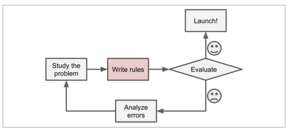
일반적인 문제 해결 절차
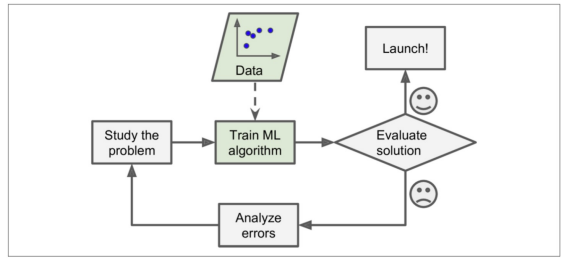
데이터 기반이라면
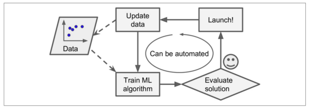
모델 스스로 데이터를 기반으로 변화에 대응 가능
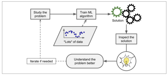
심지어 머신러닝을 통해 배우기도 가능

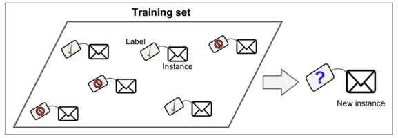
지도학습 - 분류 Classification
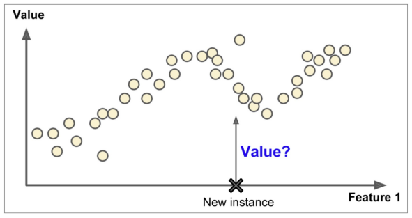
지도학습 - 회귀 Regression
비지도학습은 레이블이 없다.
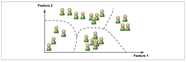
비지도 학습 - 군집
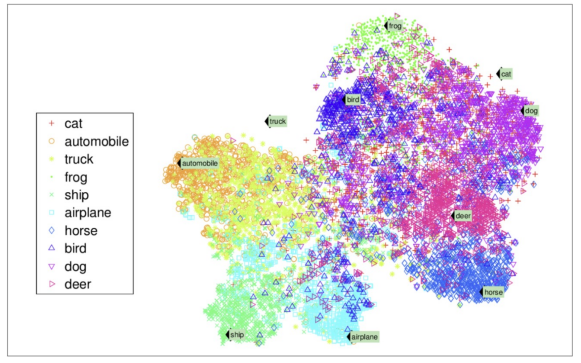
비지도 학습 - 차원축소

Regression 회귀

Hypothesis(가설, 모델)(h)

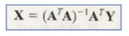
OLS : Ordinary Linear Least Square

★

# 설치

#!pip install statsmodels

# 데이터 생성

import pandas as pd

data = {'x':[1, 2, 3, 4, 5], 'y':[1, 3, 4, 6, 5]}
df = pd.DataFrame(data)
df

# 가설 생성

import statsmodels.formula.api as smf

lm_model = smf.ols(formula='y ~ x', data=df).fit()
# formula='y ~ x' : y = ax + b라는 의미

lm_model

# 결과

lm_model.params

# seaborn import

import matplotlib.pyplot as plt
import seaborn as sns

%matplotlib inline

# seaborn을 이용해서 plot

plt.figure(figsize=(12, 10))
sns.lmplot(x='x', y='y', data=df)
plt.xlim([0, 5])

잔차평가 residue : 잔차(모델과 실제 값의 차이)는 평균이 0인 정규분포를 따라야 한다. 잔차 평가는 잔차의 평균이 0이고 정규분포를 따르는 지 확인(잔차의 평균이 0이면 데이터가 굉장히 많을 때 직선에 모인다(?))

# 잔차 확인
resid = lm_model.resid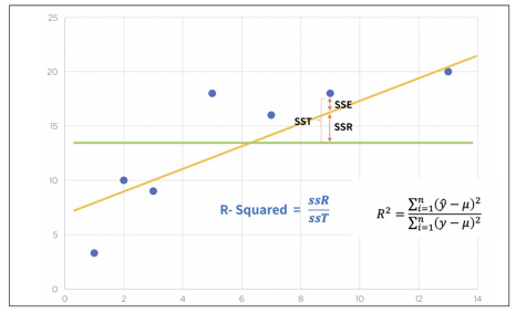
resid

결정계수 R-Squred : 예측 값과 실제 값(y)이 일치하면 결정계수는 1이 됨 (즉 결정계수가 높을 수록 좋은 모델) (참 값들의 오차 제곱의 합과 예측 값들의 평균으로부터 오차 제곱의 합이 일치할수록 좋다(?) )

# numpy로 직접 결정계수 계산

import numpy as np

mu = np.mean(df.y)
y = df.y
yhat = lm_model.predict()
np.sum((yhat - mu)**2 / np.sum((y - mu)**2))

lm_model.rsquared

# 잔차의 분포도 확인

sns.distplot(resid, color = 'black')

통계적 회귀

# import

import pandas as pd
import numpy as np
import matplotlib.pyplot as plt
import seaborn as sns

# 데이터 로드

data_url = 'https://raw.githubusercontent.com/PinkWink/ML_tutorial/master/dataset/ecommerce.csv'
data = pd.read_csv(data_url)

data

# 현재 컬럼
data.columns

# 필요 없는 컬럼 삭제

data.drop(['Email', 'Address', 'Avatar'], axis=1, inplace=True)
data.info()

# 컬럼별 boxplot
plt.figure(figsize=(12, 6))
sns.boxplot(data=data)

# 특성들만 다시 boxplot

plt.figure(figsize=(12, 6))
sns.boxplot(data=data.iloc[:,:-1])

# Label 값에 대한 boxplot

plt.figure(figsize=(12, 6))
sns.boxplot(data=data['Yearly Amount Spent'])

# pairplot으로 경향 확인
# 큰 상관관계를 보이는 것은 멤버쉽 유지 기간


plt.figure(figsize=(12, 6))
sns.pairplot(data=data)

# lmplot으로 확인

plt.figure(figsize=(12, 6))
sns.lmplot(x='Length of Membership', y='Yearly Amount Spent', data=data)

# 상관이 높은 멤버쉽 유지기간만 가지고 통계적 회귀


#R-squared : 모형 적합도, y의 분산을 각각의 변수들이 약 99.8%로 설명할 수 있음
# Adj. R-squared : 독립변수가 여러 개인 다중회귀분석에서 사용
# Prob. F-Statistic : 회귀모형에 대한 통계적 유의미성 검정.
# 이 값이 0.05 이하라면 모집단에서도 의미가 있다고 볼 수 있음

import statsmodels.api as sm

X = data['Length of Membership']
Y = data['Yearly Amount Spent']
lm = sm.OLS(Y, X).fit()
lm.summary() # 회귀리포트

# 회귀모델

pred = lm.predict(X)

sns.scatterplot(x=X, y=Y)
plt.plot(X, pred, 'r', ls = 'dashed', lw = 3);

# 참 값 vs 예측 값

sns.scatterplot(x=Y, y=pred)
plt.plot([min(Y), max(Y)], [min(Y), max(Y)], 'r', ls = 'dashed', lw = 3);

# linear model이 0부터 시작하는 것은 상수항이 없어서이다

sns.scatterplot(x=Y, y=pred)
plt.plot([min(Y), max(Y)], [min(Y), max(Y)], 'r', ls = 'dashed', lw = 3);
plt.plot([0, max(Y)], [0, max(Y)], 'b', ls = 'dashed', lw=3);
plt.axis([0, max(Y), 0, max(Y)])

# 상수항 넣기

X = np.c_[X, [1]*len(X)]
X[:5]

# 다시 모델 fit
# AIC : 값이 작을수록 좋음 (https://blog.naver.com/euleekwon/221465294530)
lm = sm.OLS(Y, X).fit()
lm.summary()

# 선형 회귀 결과
# 무조건 r-square값을 신뢰해서는 안된다. 
# https://m.blog.naver.com/PostView.naver?isHttpsRedirect=true&blogId=jiehyunkim&logNo=199212512
# https://datascienceschool.net/03%20machine%20learning/04.02%20%EC%84%A0%ED%98%95%ED%9A%8C%EA%B7%80%EB%B6%84%EC%84%9D%EC%9D%98%20%EA%B8%B0%EC%B4%88.html
pred = lm.pred = lm.predict(X)

sns.scatterplot(x=X[:,0], y=Y)
plt.plot(X[:,0], pred, 'r', ls = 'dashed', lw = 3)

# 참 값 vs 예측 값

pred = lm.predict(X)

sns.scatterplot(x=Y, y=pred)
plt.plot([min(Y), max(Y)], [min(Y), max(Y)], 'r', ls = 'dashed', lw = 3)

# 데이터 분리 후

from sklearn.model_selection import train_test_split

X = data.drop('Yearly Amount Spent', axis=1)
y = data['Yearly Amount Spent']

X_train, X_test, y_train, y_test = train_test_split(X, y, test_size= 0.3, random_state=13)

# 네 개의 컬럼을 모두 변수로 보고 회귀

import statsmodels.api as sm

lm = sm.OLS(y_train, X_train).fit()
lm.summary()

# 참 값 vs 예측 값

pred = lm.predict(X_test)

sns.scatterplot(x=y_test, y=pred)
plt.plot([min(y_test), max(y_test)], [min(y_test), max(y_test)], 'r', ls = 'dashed', lw = 3)

Cost Function 손으로 이해하는 cost function

에러를 제곱하는 이유는 부호를 없애기 위함. 그렇기 때문에 절대값을 사용하는 경우도 있다
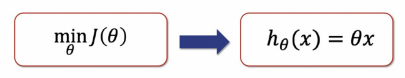
에러의 제곱을 구하고 평균을 구한다 ← Cost Function
Cost Function을 최소화할 수 있으면 최적의 직선을 찾을 수 있다

import numpy as np

a = np.poly1d([1, 1])
b = np.poly1d([1, -1])
a, b

# poly1d : 다항식 계산 https://numpy.org/doc/stable/reference/generated/numpy.poly1d.html
a*b

np.poly1d([2, -1])**2 + np.poly1d([3, -5])**2 + np.poly1d([5, -6])**2

# 최소값 찾기

#!pip install sympy

# Symbolic 연산 가능

import sympy as sym

th = sym.Symbol('theta')
diff_th = sym.diff(38*th**2 - 94*th + 62, th)
diff_th

94/76

Cost Function, Gradient Descent

Cost Function : 비용함수, 최소값을 찾아야 한다 (참고 : https://wikidocs.net/4289)
Gradient Descent : 경사 하강 알고리즘은 비용 함수 J(θ(0),θ(1))를 최소화 하는 θ를 구하는 알고리즘 (참고 : https://box-world.tistory.com/7)
Learning Rate : 학습률 (alpha는 얼마만큼 theta를 갱신할 것인지를 설정하는 값).
학습률이 작다면 최솟값을 찾으러 가는 간격이 작게됨. 여러번 갱신해야 하나, 대신 최솟값에 잘 도달할 수 있다.
학습률이 크다면 최솟값을 찾으러 가는 간격이 크게됨. 최솟값을 찾았다면 갱신 횟수는 상대적으로 적을 수 있으나, 수렴하지 않고 진동할 수 있다.