😢 스터디노트 (Machine Learning 5)

Model Evaluation - 모델 평가 개념

• 데이터 수집/가공/변환 → 모델 학습/예측 → 모델평가 반복

• 다양한 모델, 다양한 파라미터를 두고, 상대적으로 비교한다.
  - 회귀모델들은 실제 값과 에러치를 가지고 계산
  - 분류 모델의 평가 항목이 조금 많다 (정확도, 오차행렬, 정밀도, 재현율, F1 score, ROC AUC 등등...)
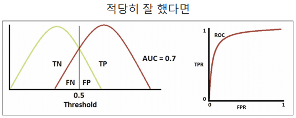
  - 이진 분류 모델의 평가
  - TP True Positive : 실제 Positive를 Positive라고 맞춘 경우
  - FN False Negative : 실제 Positive를 Negative라고 틀리게 예측한 경우
  - TN True Negative : 실제 Negative를 Negative라고 맞춘 경우
  - FP False Positive : 실제 Negative를 Positive라고 틀리게 예측한 경우

• Accuracy : 전체 데이터 중에 맞게 예측한 것의 비율

• Precision : 참(양성)이라고 예측한 것 중에서 실제 참(양성)의 비율 (precision = TP / (TP + FP)) (ex) 스팸메일이라고 예측했는데 스팸이 아닌 경우 곤란하다)

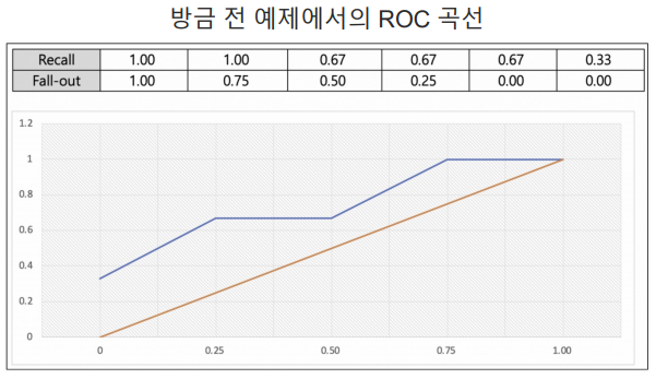
• ★ RECALL(TPR TRUE POSITIVE RATIO) : 참인 데이터들 중에서 참이라고 예측한 것 (recall = TP / (TP + FN)) ★

• FALL_OUT(FPR FALSE POSITIVE RATIO) : 실제 양성이 아닌데, 양성이라고 잘못 예측한 경우
  
  
  

---

• 분류모델은 그 결과를 속할 비율(확률)을 반환한다.
  - 이진분류에서는 비율에서 threshold를 0.5라고 하고 0, 1로 결과를 반영했다.
  
  

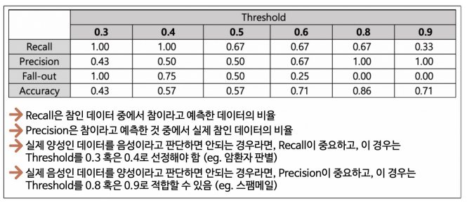
• ★ Recall과 Precision은 서로 영향을 주기 때문에 한 쪽을 극단적으로 높게 설정해서는 안된다.
  
  
  

---

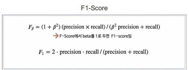
F1 - Score

- F1 - Score : Recall과 Precision을 결합한 지표. Recall과 Precision이 어느 한쪽으로 치우치지 않고 둘 다 높은 값을 가질 수록 높은 값을 가짐

---

Model Evaluation - ROC와 AUC

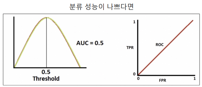
• ROC 곡선 :
  ※ FPR : FALL_OUT(FPR FALSE POSITIVE RATIO)
  ※ TPR : RECALL(TPR TRUE POSITIVE RATIO)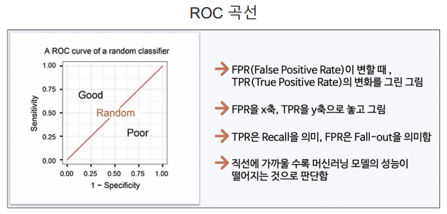

  
  
  
  

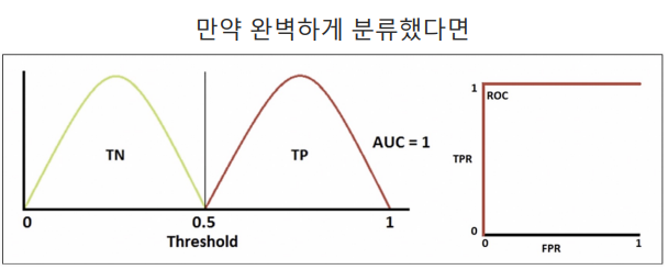
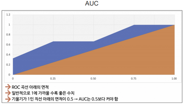
• AUC : ROC 곡선의 아래의 면적. 일반적으로 1에 가까울수록 좋은 수치. 기울기가 1인 직선 아래의 면적이 0.5 → AUC는 0.5보다 커야 함

  
  

---

Model Evaluation - ROC 커브 그려보기

# 다시 와인 맛 분류하던 데이터로\
# 데이터 읽기

import pandas as pd

red_url = 'https://raw.githubusercontent.com/PinkWink/ML_tutorial/master/dataset/winequality-red.csv'
white_url = 'https://raw.githubusercontent.com/PinkWink/ML_tutorial/master/dataset/winequality-white.csv'

red_wine = pd.read_csv(red_url, sep=';')
white_wine = pd.read_csv(white_url, sep=';')

red_wine['color'] = 1
white_wine['color'] = 0

wine = pd.concat([red_wine, white_wine])
wine['taste'] = [1 if grade > 5 else 0 for grade in wine['quality']]

X = wine.drop(['taste', 'quality'], axis=1)
Y = wine['taste']

# 간단히 결정나무 적용하기

from sklearn.model_selection import train_test_split
from sklearn.tree import DecisionTreeClassifier
from sklearn.metrics import accuracy_score

X_train, X_test, Y_train, Y_test = train_test_split(X, Y, test_size=0.2, random_state=13)

wine_tree = DecisionTreeClassifier(max_depth=2, random_state=13)
wine_tree.fit(X_train, Y_train)

y_pred_tr = wine_tree.predict(X_train)
y_pred_test = wine_tree.predict(X_test)

print('Train Acc : ', accuracy_score(Y_train, y_pred_tr))
print('Test Acc : ', accuracy_score(Y_test, y_pred_test))

# 각 수치 구해보기

from sklearn.metrics import (accuracy_score, precision_score, 
                             recall_score, f1_score, roc_auc_score, roc_curve)

print('Accuracy : ', accuracy_score(Y_test, y_pred_test))
print('Recall : ', recall_score(Y_test, y_pred_test))
print('Precision : ', precision_score(Y_test, y_pred_test))
print('AUC Score : ', roc_auc_score(Y_test, y_pred_test))
print('F1 Score : ', f1_score(Y_test, y_pred_test))

wine_tree.predict_proba(X_test) # 0일 확률, 1일 확률

roc_curve(Y_test, pred_proba)

# ROC 커브 그리기

import matplotlib.pyplot as plt
%matplotlib inline

pred_proba = wine_tree.predict_proba(X_test)[:, 1]
fpr, tpr, thresholds = roc_curve(Y_test, pred_proba)

fpr

tpr

thresholds

plt.figure(figsize=(10, 8))
plt.plot([0, 1], [0, 1], 'r', ls = 'dashed') # 0, 0 ~ 1, 1 사이의 그래프가 그려짐, 보조선 역할
plt.plot(fpr, tpr)
plt.grid()
plt.show()

---

수학이 기초 - 함수

• 다항함수

  

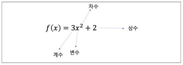
# 다항함수

import numpy as np
import matplotlib.pyplot as  plt

x = np.linspace(-3, 2, 100)
y = 3*x**2 + 2

x

y

plt.figure(figsize=(12, 8))
plt.plot(x, y)
plt.xlabel('$x$')
plt.ylabel('$y$')
plt.show()

# style

import matplotlib as mpl

mpl.style.use('seaborn-whitegrid')

plt.figure(figsize=(12, 8))
plt.plot(x, y)
plt.xlabel('$x$', fontsize = 25)
plt.ylabel('$y$', fontsize = 25)
plt.show()

# 다항함수의 x 축 방향 이동

x = np.linspace(-5, 5, 100)
y1 = 3*x**2 + 2
y2 = 3*(x+1)**2 + 2

# plot

plt.figure(figsize=(12, 8))
plt.plot(x, y1, lw = 2, ls = 'dashed', label = '$y=3x^2 + 2$')
plt.plot(x, y2, label = '$y=3(x+1)^2 + 2$')
plt.legend(fontsize = 15)
plt.xlabel('$x$', fontsize = 25)
plt.ylabel('$y$', fontsize = 25)
plt.show()

---

• 지수함수

  

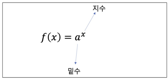
# 지수함수
# 지수함수를 파악하기 위해 다양한 경우

x = np.linspace(-2, 2, 100)
a11, a12, a13 = 2, 3, 4
y11, y12, y13 = a11**x, a12**x, a13**x

a21, a22, a23 = 1/2, 1/3, 1/4
y21, y22, y23 = a21**x,  a22**x, a23**x

# 그래프

fig, ax = plt.subplots(1, 2, figsize=(12, 6))

ax[0].plot(x, y11, color = 'k', label = r'$2^x$')
ax[0].plot(x, y12, '--', color = 'k', label = r'$3^x$')
ax[0].plot(x, y13, ':', color = 'k', label = r'$4^x$')

ax[0].legend(fontsize = 20)

ax[1].plot(x, y21, color = 'k', label = r'$(1/2)^x$')
ax[1].plot(x, y22, '--', color = 'k', label = r'$(1/3)^x$')
ax[1].plot(x, y23, ':', color = 'k', label = r'$(1/4)^x$')

ax[1].legend(fontsize = 20)

x = np.linspace(0, 10)

plt.figure(figsize = (6, 6))

plt.plot(x, x**2, '--', color = 'k', label = r'$x^2$')
plt.plot(x, 2**x, color = 'k', label = r'$2^x$')

plt.legend(loc = 'center left', fontsize = 25)
plt.xlabel('$x$', fontsize = 25)
plt.ylabel('$y$', fontsize = 25)

plt.show()

---

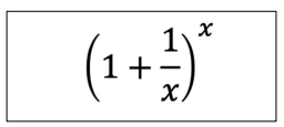
x = np.array([10, 100, 1000, 10000, 100000])
(1 + 1/x)**x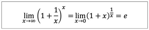

---

---

• 로그함수

  

# 로그함수를 그리기 위한 데이터

def log(x, base):
    return np.log(x)/np.log(base)

x1 = np.linspace(0.0001, 5, 1000)
x2 = np.linspace(0.01, 5, 100)

y11, y12 = log(x1, 10), log(x2, np.e)
y21, y22 = log(x1, 1/10), log(x2, 1/np.e)

# 그리기 위한 준비

fig, ax = plt.subplots(1, 2, figsize = (12, 6))

ax[0].plot(x1, y11, label = r'$log_{10} x$', color = 'k')
ax[0].plot(x2, y12, '--', label = r'$log_{e} x$', color = 'k')

ax[0].set_xlabel('$x$', fontsize = 25)
ax[0].set_ylabel('$y$', fontsize = 25)
ax[0].legend(fontsize = 20, loc = 'lower right')

ax[1].plot(x1, y21, label = r'$log_{10} x$', color = 'k')
ax[1].plot(x2, y22, '--', label = r'$log_{1/e} x$', color = 'k')

ax[1].set_xlabel('$x$', fontsize = 25)
ax[1].set_ylabel('$y$', fontsize = 25)
ax[1].legend(fontsize = 20, loc = 'upper right')

plt.show()

---

• 시그모이드 Sigmoid : 0 ~ 1사이의 값을 가짐

  

# 시그모이드

z = np.linspace(-10, 10, 100)
sigma = 1/(1+np.exp(-z))

plt.figure(figsize=(12, 8))
plt.plot(z, sigma)
plt.xlabel('$z$', fontsize = 25)
plt.ylabel('$\sigma(z)$', fontsize = 25)
plt.show()

---

수학이 기초 - 함수의 표현

• 벡터의 표현

  

• 단일 변수 스칼라 표현

  

• 다중 변수 스칼라 함수

  

• 다변수 벡터 함수

  

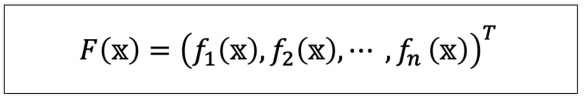
다면수 벡터함수 예제)

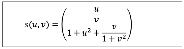
# 다변수 벡터함수 예제

u = np.linspace(0, 1, 30)
v = np.linspace(0, 1, 30)

U, V = np.meshgrid(u, v)
X = U
Y = V

U, V = np.meshgrid(u, v)
U, V

Z = (1 + U**2) + (V/(1+V**2))
z

t = np.linspace(0, 4, 3)
p = np.linspace(0, 4, 3)
T, P = np.meshgrid(t, p)
T, P

# 그리기

fig = plt.figure(figsize=(7, 7))
ax = plt.axes(projection = '3d')
ax.xaxis.set_tick_params(labelsize = 15)
ax.yaxis.set_tick_params(labelsize = 15)
ax.zaxis.set_tick_params(labelsize = 15)
ax.set_xlabel(r'$x$', fontsize = 20)
ax.set_ylabel(r'$y$', fontsize = 20)
ax.set_xlabel(r'$z$', fontsize = 20)

ax.scatter3D(U, V, Z, marker = '.', color = 'gray')

plt.show()

# 함수 합성 예제

x = np.linspace(-4, 4, 100)
y = x**3 - 15*x + 30
z = np.log(y)

# 함수 생김새

fig, ax = plt.subplots(1, 2, figsize = (12, 6))

ax[0].plot(x, y, label=r'$x^3 - 15x + 30$', color = 'k')
ax[0].legend(fontsize = 18)

ax[1].plot(y, z, label=r'$\log(y)$', color = 'k')
ax[1].legend(fontsize = 18)

plt.show()

# 합성한 것 생김새

fig, ax = plt.subplots(1, 2, figsize = (12, 6))

ax[0].plot(x, z,'--', label=r'$\log(f(x))$', color = 'k')
ax[0].legend(fontsize = 18)

ax[1].plot(x, y, label=r'$x^3 - 15x + 30$', color = 'k')
ax[1].legend(fontsize = 18)

ax_tmp = ax[1].twinx() # x축을 하나 더 만들어라
ax_tmp.plot(x, z, '--', label = r'$\log(f(x))$', color = 'k') # 만든 x축에 맞춰 그래프를 그려라

plt.show()

---

box plot

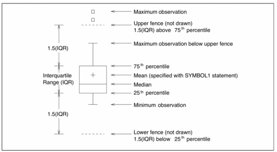
# 간단한 데이터

sample = [1, 7, 9, 16, 36, 39, 45, 45, 46, 48, 51, 100, 101]
tmp_y = [1]*len(sample)
tmp_y

# plot

plt.figure(figsize=(12, 4))
plt.scatter(sample, tmp_y)
plt.grid()
plt.show()

# 지표를 찾는 법

np.median(sample)

np.percentile(sample, 25)

np.percentile(sample, 75) - np.percentile(sample, 25)

iqr = np.percentile(sample, 75) - np.percentile(sample, 25)
iqr * 1.5

# 그리기

q1 = np.percentile(sample, 25)
q2 = np.median(sample)
q3 = np.percentile(sample, 75)
iqr = q3 - q1
upper_fence = q3 + iqr*1.5
lower_fence = q1 - iqr-1.5

plt.figure(figsize=(12, 4))
plt.scatter(sample, tmp_y)
plt.axvline(x=q1, color='black')
plt.axvline(x=q2, color='red')
plt.axvline(x=q3, color='black')
plt.axvline(x=upper_fence, color='black', ls = 'dashed')
plt.axvline(x=lower_fence, color='black', ls = 'dashed')
plt.grid()
plt.show()

# framework 이용

import seaborn as sns

plt.figure(figsize=(12, 4))
sns.boxenplot(sample)
plt.grid()
plt.show()

어렵..

💻 출처 : 제로베이스 데이터 취업 스쿨