Below, I'll provide a SAS example that mirrors the process you described, integrating the cloud deployment and interactivity concepts from your Azure-based Python request. I'll assume we're working with a dataset resembling Immunization Information Systems or National Healthcare Safety Network Long-Term Care data. Since SAS doesn’t natively support Azure Event Hubs or Streamlit-like interactivity, I’ll adapt the process to use SAS with Azure SQL for data storage and retrieval, and suggest ways to extend it for dynamic updates and interactivity.
SAS Example: Vaccination Coverage and Survival Analysis
Step 1: Setup and Assumptions
Dataset: Simulated vaccination data with columns: patient_id, age, gender, comorbidity_flag, vaccination_date, vaccine_received, state, income_category.
Azure SQL: Data stored in an Azure SQL Database (e.g., VaccineDB).
SAS Environment: SAS 9.4 or SAS Viya with access to ODBC for Azure SQL.
SAS Code
sas
/ Step 1: Connect to Azure SQL Database /
libname azuresql odbc dsn="AzureSQLDSN" schema=dbo;
/ Configure ODBC DSN 'AzureSQLDSN' in SAS with connection string:
DRIVER={ODBC Driver 17 for SQL Server};
SERVER=yourserver.database.windows.net;
DATABASE=VaccineDB;
UID=youruser;
PWD=yourpass /
/ Step 2: Import and Clean Data /
proc sql;
create table vaccine_raw as
select patient_id, age, gender, comorbidity_flag, vaccination_date, vaccine_received, state, income_category
from azuresql.VaccineData
where vaccination_date is not null; / Basic filter for missing dates /
quit;
/ Data Cleaning: Remove unrealistic values /
data vaccine_cleaned;
set vaccine_raw;
/ Remove extreme ages /
if age < 0 or age > 120 then delete;
/ Ensure gender is valid /
if gender not in ('M', 'F', 'Other') then gender = 'Unknown';
/ Convert vaccination_date to SAS date /
vacc_date_num = input(vaccination_date, yymmdd10.);
format vacc_date_num date9.;
/ Flag for survival analysis /
if vaccine_received = 1 and vacc_date_num is not missing then time_to_vacc = vacc_date_num - '01JAN2020'd;
else time_to_vacc = .; / Missing if not vaccinated /
run;
/ Step 3: Calculate Vaccination Coverage /
proc freq data=vaccine_cleaned;
tables vaccine_received income_category / out=coverage_out (drop=percent);
where vacc_date_num between '01JAN2024'd and '31DEC2024'd; / Specific time frame */
run;
proc sql;
create table coverage_rates as
select income_category,
sum(case when vaccine_received = 1 then count else 0 end) as vaccinated,
sum(count) as total,
calculated vaccinated / calculated total * 100 as vacc_rate
from coverage_out
group by income_category;
quit;
proc print data=coverage_rates;
title "Vaccination Coverage by Income Category (2024)";
run;
/ Step 4: Survival Analysis (Kaplan-Meier) /
proc lifetest data=vaccine_cleaned plots=survival(atrisk);
time time_to_vacc vaccine_received(0); / 0 = censored (not vaccinated) /
strata age_group; / Assuming age_group is derived below /
/ Derive age groups */
if age < 18 then age_group = '0-17';
else if age < 65 then age_group = '18-64';
else age_group = '65+';
ods output survivalplot=surv_data;
title "Time to Vaccination by Age Group";
run;
/ Step 5: Cox Proportional Hazards Model /
proc phreg data=vaccine_cleaned;
class gender (ref='F') income_category (ref='Medium') comorbidity_flag (ref='0');
model time_to_vacc * vaccine_received(0) = age gender comorbidity_flag income_category / risklimits;
title "Cox Model: Factors Affecting Time to Vaccination";
run;
/ Step 6: Insights into Trends and Disparities /
/ Example: Summarize by state and gender /
proc means data=vaccine_cleaned n mean;
class state gender;
var vacc_rate;
output out=disparity_summary mean=vacc_mean;
run;
proc print data=disparity_summary;
title "Vaccination Rate Disparities by State and Gender";
run;
/ Step 7: Export Cleaned Data /
proc export data=vaccine_cleaned
outfile="C:\path\to\export\vaccine_cleaned.csv"
dbms=csv replace;
run;
/ Optional: Write back to Azure SQL for further use /
proc sql;
create table azuresql.VaccineCleaned as
select * from vaccine_cleaned;
quit;
Explanation of Steps in SAS
Connection to Azure SQL:
Uses libname with an ODBC connection to pull data from Azure SQL. Configure the DSN in your SAS environment.
Data Cleaning:
Filters out missing vaccination_date, removes extreme ages (<0 or >120), and standardizes gender.
Converts vaccination_date to a SAS date and calculates time_to_vacc as days since a baseline (e.g., Jan 1, 2020).
Vaccination Coverage:
proc freq calculates frequencies, and proc sql computes coverage rates by income_category for 2024.
Output: A table showing total population, vaccinated count, and percentage.
Survival Analysis (Kaplan-Meier):
proc lifetest models time to vaccination, stratified by age_group.
Plots survival curves (probability of remaining unvaccinated) with at-risk counts.
Cox Proportional Hazards Model:
proc phreg estimates hazard ratios for age, gender, comorbidity_flag, and income_category.
Identifies factors influencing vaccination timing (e.g., higher comorbidity may accelerate vaccination).
Insights and Disparities:
proc means summarizes vaccination rates by state and gender to highlight disparities.
Export:
Exports cleaned data to CSV and optionally writes back to Azure SQL for downstream use.
Adapting for Azure Deployment and Interactivity
Dynamic Updates
SAS doesn’t natively support real-time streaming like Azure Event Hubs. Instead:
Batch Updates: Schedule the SAS job to run periodically (e.g., daily) using SAS Schedule Manager or Azure Data Factory:
sas
/ Azure Data Factory Trigger Example /
/ Pipeline runs this SAS script via a Custom Activity /
Pseudo-Real-Time: Use an Azure Function to insert new data into Azure SQL, and SAS queries the updated table:
python
Azure Function (from previous Python example)
def main(event: str):
data = json.loads(event.get_body().decode('utf-8'))
# Insert into VaccineData tableInteractivity (Dropdown Filters)
SAS lacks a native Streamlit-like interface, but you can:
SAS Stored Process:
Convert the script into a stored process with parameters for filters:
sas
%global gender income state;
proc sql;
create table filtered_data as
select from vaccine_cleaned
where gender in (&gender) and income_category in (&income) and state in (&state);
quit;
Deploy on SAS Server and access via SAS Web Application with dropdowns.
SAS Visual Analytics:
Import vaccine_cleaned into SAS Viya.
Create a report with filters for gender, income_category, state, etc., and dynamic Kaplan-Meier plots.
Kaplan-Meier Dynamic Updates
Rerun proc lifetest whenever new data is loaded:
sas
proc lifetest data=vaccine_cleaned plots=survival(atrisk);
time time_to_vacc vaccine_received(0);
strata income_category; / Dynamic stratification /
run;
In SAS Visual Analytics, link this to a data refresh trigger.
Example with Filters in SAS Stored Process
sas
/ Stored Process: Vaccination Analysis with Filters /
%global gender income state;
libname azuresql odbc dsn="AzureSQLDSN" schema=dbo;
proc sql;
create table filtered_data as
select * from azuresql.VaccineData
where gender in (&gender) and income_category in (&income) and state in (&state)
and age between 0 and 120;
quit;
proc lifetest data=filtered_data plots=survival(atrisk);
time time_to_vacc * vaccine_received(0);
strata income_category;
run;
proc phreg data=filtered_data;
class gender income_category;
model time_to_vacc * vaccine_received(0) = age gender;
run;
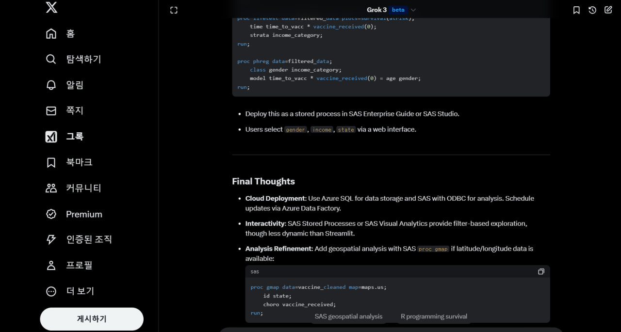
Deploy this as a stored process in SAS Enterprise Guide or SAS Studio.
Users select gender, income, state via a web interface.
Final Thoughts
Cloud Deployment: Use Azure SQL for data storage and SAS with ODBC for analysis. Schedule updates via Azure Data Factory.
Interactivity: SAS Stored Processes or SAS Visual Analytics provide filter-based exploration, though less dynamic than Streamlit.
Analysis Refinement: Add geospatial analysis with SAS proc gmap if latitude/longitude data is available:
sas
proc gmap data=vaccine_cleaned map=maps.us;
id state;
choro vaccine_received;
run;
Let me know if you need help configuring the Azure-SAS connection, deploying a stored process, or integrating additional variables!
Example:
I’ll provide an explanation of patient-reported outcome (PRO) measurement development and patient preference studies, focusing on the methodologies you mentioned: Classical Test Theory (CTT), Item Response Theory (IRT), trade-off methods, and Discrete Choice Experiments (DCE). These are critical in health research for understanding patient experiences and preferences, which can tie into your vaccination analysis by assessing outcomes like vaccine satisfaction or hesitancy drivers.
Patient-Reported Outcome (PRO) Measurement Development
PROs are direct reports from patients about their health status, quality of life, or treatment experiences, without clinician interpretation. Developing PRO measures involves creating reliable, valid, and responsive instruments (e.g., questionnaires). Two foundational psychometric approaches are Classical Test Theory (CTT) and Item Response Theory (IRT).
1. Classical Test Theory (CTT)
CTT is a traditional framework for designing and evaluating PRO instruments based on observable scores.
Core Concept:
Observed Score = True Score + Error
The goal is to estimate the "true" underlying construct (e.g., pain, satisfaction) while minimizing measurement error.
Key Steps in Development:
Item Generation: Develop questions based on patient interviews, literature, or expert input (e.g., "How satisfied are you with your vaccine?").
Reliability: Assess consistency using:
Cronbach’s Alpha: Measures internal consistency (e.g., α > 0.7 is acceptable).
Test-Retest Reliability: Correlates scores over time for stability.
Validity: Ensure the instrument measures what it intends:
Content Validity: Items cover all relevant aspects (e.g., vaccine side effects, convenience).
Construct Validity: Correlates with related measures (e.g., satisfaction vs. quality of life).
Criterion Validity: Predicts external outcomes (e.g., vaccine uptake).
Scoring: Sum or average item responses (e.g., 1-5 Likert scale).
Example in SAS:
sas
proc corr data=vaccinepro alpha;
var item1 item2 item3; / Satisfaction items /
run;
/ Cronbach’s Alpha to check reliability /
Strengths: Simple, widely understood, computationally light.
Limitations: Assumes all items are equally difficult and doesn’t account for individual differences in response patterns.
2. Item Response Theory (IRT)
IRT is a modern psychometric approach that models the relationship between a latent trait (e.g., vaccine hesitancy) and item responses, offering more granularity than CTT.
Core Concept:
Probability of a response (e.g., "Yes" to "Would you recommend this vaccine?") depends on the patient’s latent trait level (θ) and item parameters (difficulty, discrimination).
Common model: 2-Parameter Logistic (2PL):
P(X_i = 1 | \theta) = \frac{1}{1 + e^{-a_i(\theta - b_i)}}
a_i
: Discrimination (how well the item differentiates high vs. low trait levels).
b_i
: Difficulty (trait level needed for 50% chance of endorsing the item).
Key Steps in Development:
Item Calibration: Fit an IRT model to estimate
a_i
and
b_i
using patient responses.
Fit Assessment: Check model assumptions (e.g., unidimensionality) with factor analysis or fit statistics.
Scoring: Estimate
\theta
for each patient (e.g., hesitancy score).
Item Selection: Choose items with high discrimination and a range of difficulties.
Example in SAS (Using PROC IRT):
sas
proc irt data=vaccine_pro;
model item1-item5 / rescale=1.7; / 5 items on vaccine attitudes /
var item1-item5;
run;
/ Outputs item parameters and theta scores /
Strengths: Adaptive (supports computerized adaptive testing), accounts for item difficulty, precise at individual level.
Limitations: Requires larger samples, assumes unidimensionality, computationally intensive.
CTT vs. IRT:
CTT is better for quick, simple scales; IRT excels for adaptive, precise measures (e.g., tailoring questions to hesitancy levels).
PRO Application
For vaccination, a PRO might measure satisfaction or side effect burden. Development involves:
Qualitative phase: Patient focus groups to identify domains (e.g., trust, access).
Quantitative phase: Pilot test with CTT/IRT to refine items.
Validation: Compare against outcomes like vaccination rates.
Patient Preference Studies
Preference studies assess how patients value different aspects of treatments (e.g., vaccine efficacy vs. side effects). Two common methods are trade-off methods and Discrete Choice Experiments (DCE).
1. Trade-Off Methods
Trade-off methods elicit preferences by asking patients to weigh attributes against each other.
Types:
Threshold Technique: Identify the minimum benefit (e.g., efficacy %) needed to accept a risk (e.g., side effects).
Standard Gamble: Choose between a certain outcome (e.g., mild side effects) and a gamble (e.g., 90% chance of no side effects, 10% severe).
Time Trade-Off (TTO): Trade years of life for a better health state (e.g., living 9 years without side effects vs. 10 with).
Process:
Define attributes (e.g., vaccine efficacy, side effect severity, administration mode).
Present scenarios (e.g., "Would you accept a 5% side effect risk for 95% efficacy?").
Analyze trade-offs to estimate utility weights.
Example:
Patients might trade 1 year of life to avoid severe vaccine side effects, revealing preference strength.
Analysis in SAS:
sas
proc means data=tradeoff_data;
var efficacy side_effect_risk;
output out=tradeoff_summary mean=;
run;
Strengths: Intuitive, captures risk tolerance.
Limitations: Hypothetical, cognitively demanding.
2. Discrete Choice Experiments (DCE)
DCEs present patients with choice sets of hypothetical options, each defined by attributes and levels, to infer preferences.
Core Concept:
Patients choose between options (e.g., Vaccine A: 90% efficacy, mild side effects vs. Vaccine B: 80% efficacy, no side effects).
Preferences modeled with random utility theory:
U{ij} = V{ij} + \epsilon{ij}
V{ij}
: Systematic utility (e.g.,
\beta_1 \cdot efficacy + \beta_2 \cdot side_effects
).
\epsilon{ij}
: Random error.
Key Steps:
Attribute Selection: Identify factors (e.g., efficacy, cost, side effects).
Level Assignment: Define ranges (e.g., efficacy: 70%, 85%, 95%).
Design Choice Sets: Use fractional factorial design to reduce combinations (e.g., SAS proc factex).
Data Collection: Patients select preferred options.
Analysis: Fit a conditional logit or mixed logit model to estimate
\beta
coefficients.
Example in SAS:
sas
/ Generate DCE design /
proc factex;
factors efficacy side_effects cost;
levels 3 2 3; / efficacy: 70, 85, 95; side_effects: mild, severe; cost: $0, $10, $20 /
output out=dce_design;
run;
/ Simulate patient choices /
data dce_data;
set dce_design;
choice = (efficacy 0.05 - side_effects 0.3 - cost 0.01 > 0); / Simplified utility */
run;
/ Analyze with conditional logit /
proc logistic data=dcedata descending;
model choice = efficacy side_effects cost / link=logit;
run;
Output: Coefficients show preference strength (e.g.,
\beta{efficacy} = 0.05
means 1% efficacy increase raises utility by 0.05).
Strengths: Realistic, quantifies attribute importance, supports policy simulation.
Limitations: Assumes rational choice, complex design.
Application to Vaccination
Trade-Off: “Would you accept a 10% side effect risk for a 95% effective vaccine?”
DCE: Compare Vaccine A (95% efficacy, $20, injection) vs. Vaccine B (85% efficacy, $0, nasal). Results inform vaccine promotion strategies.
Integration with Vaccination Analysis
PRO: Develop a scale for vaccine satisfaction using IRT, then correlate
\theta
scores with vaccination rates in your Azure data.
Preference: Use DCE to identify why patients prefer one vaccine brand, linking results to survival curves (e.g., faster uptake for preferred brands).
Let me know if you’d like SAS code for a specific PRO or preference method tied to your dataset!