DL - MNIST using CNN

DL - MNIST using CNN

import tensorflow as tf

mnist = tf.keras.datasets.mnist

(x_train,y_train), (x_test,y_test) = mnist.load_data()
X_train,X_test = x_train/255, x_test/255 #픽셀 max 255로 나누기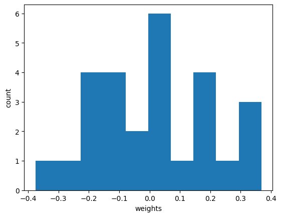![](https://velog.velcdn.com/images/sjm0321/post/6e639762-1a59-4853-a716-1e61824ec400/image.png)


X_train = X_train.reshape((60000,28,28,1))
X_test = X_test.reshape((10000,28,28,1))

from tensorflow.keras import layers, models

model = models.Sequential([
    layers.Conv2D(3,kernel_size=(3,3),strides=(1,1), #채널 3, 커널사이즈(3,3)
                  padding='same',activation='relu',
                  input_shape=(28,28,1)),
    layers.MaxPool2D(pool_size=(2,2),strides=(2,2)),
    layers.Dropout(0.25),
    layers.Flatten(),
    layers.Dense(1000,activation='relu'),
    layers.Dense(10,activation='softmax')
])

model.summary()

Model: "sequential"
_________________________________________________________________
 Layer (type)                Output Shape              Param #   
=================================================================
 conv2d (Conv2D)             (None, 28, 28, 3)         30        
                                                                 
 max_pooling2d (MaxPooling2D  (None, 14, 14, 3)        0         
 )                                                               
                                                                 
 dropout (Dropout)           (None, 14, 14, 3)         0         
                                                                 
 flatten (Flatten)           (None, 588)               0         
                                                                 
 dense (Dense)               (None, 1000)              589000    
                                                                 
 dense_1 (Dense)             (None, 10)                10010     
                                                                 
=================================================================
Total params: 599,040
Trainable params: 599,040
Non-trainable params: 0
_________________________________________________________________

# 구성한 layers들 호출
model.layers

[<keras.layers.convolutional.Conv2D at 0x241221fd220>,
 <keras.layers.pooling.MaxPooling2D at 0x24122213bb0>,
 <keras.layers.core.dropout.Dropout at 0x2413f98a130>,
 <keras.layers.core.flatten.Flatten at 0x2413f98a460>,
 <keras.layers.core.dense.Dense at 0x2413f98a5b0>,
 <keras.layers.core.dense.Dense at 0x2413f98a820>]

#아직 학습하지 않은 conv레이어 웨이트 평균 (랜덤값 상태)
conv = model.layers[0] #layers첫번째, convolutional.Conv2D
conv_weights = conv.weights[0].numpy()
conv_weights.mean(), conv_weights.std()

(0.014136259, 0.18722035)

import matplotlib.pyplot as plt

plt.hist(conv_weights.reshape(-1,1))
plt.xlabel('weights')
plt.ylabel('count')
plt.show()

# conv_weights  / 채널 3, 커널사이즈(3,3)
fig,ax = plt.subplots(1,3,figsize=(15,5))
for i in range(3):
    ax[i].imshow(conv_weights[:,:,0,i], vmin=-0.5, vmax=0.5) #3개 같이 비교하고싶을때 vmin,max 꼭 지정해주기
    ax[i].axis('off')
    
plt.show()

%%time
model.compile(optimizer='adam',loss='sparse_categorical_crossentropy',
             metrics=['accuracy'])
hist = model.fit(X_train,y_train,epochs=5, verbose=1,
                validation_data=(X_test,y_test))

Epoch 1/5
1875/1875 [==============================] - 9s 5ms/step - loss: 0.2364 - accuracy: 0.9280 - val_loss: 0.0833 - val_accuracy: 0.9732
Epoch 2/5
1875/1875 [==============================] - 10s 5ms/step - loss: 0.1051 - accuracy: 0.9667 - val_loss: 0.0638 - val_accuracy: 0.9799
Epoch 3/5
1875/1875 [==============================] - 11s 6ms/step - loss: 0.0800 - accuracy: 0.9744 - val_loss: 0.0569 - val_accuracy: 0.9808
Epoch 4/5
1875/1875 [==============================] - 12s 6ms/step - loss: 0.0661 - accuracy: 0.9788 - val_loss: 0.0529 - val_accuracy: 0.9826
Epoch 5/5
1875/1875 [==============================] - 12s 6ms/step - loss: 0.0565 - accuracy: 0.9819 - val_loss: 0.0481 - val_accuracy: 0.9842
CPU times: total: 3min 57s
Wall time: 54.3 s

# 학습 후 conv filter 변화 
fig,ax = plt.subplots(1,3,figsize=(15,5))
for i in range(3):
    ax[i].imshow(conv_weights[:,:,0,i], vmin=-0.5, vmax=0.5) 
    ax[i].axis('off')
    
plt.show()

train 0번 데이터 = 5

plt.imshow(X_train[0],cmap='gray');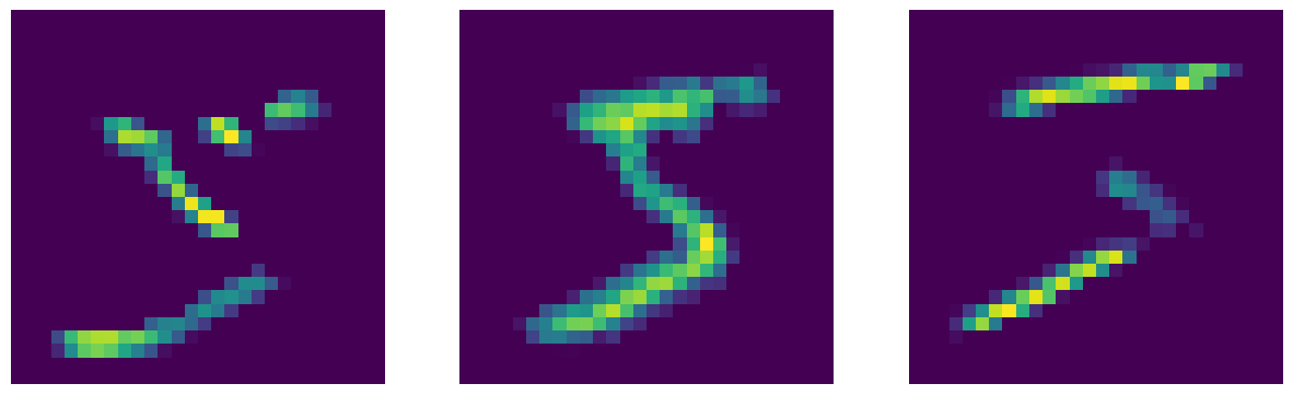

conv레이어에서 출력을 뽑는다.
모델의 input과 0번layer의 아웃풋을 모델로 연결
(fit 되어있는 상태라 weights는 고정 상태)

inputs = X_train[0].reshape(-1,28,28,1)
conv_layer_output = tf.keras.Model(model.input,model.layers[0].output)
conv_layer_output.summary()

Model: "model"
_________________________________________________________________
 Layer (type)                Output Shape              Param #   
=================================================================
 conv2d_input (InputLayer)   [(None, 28, 28, 1)]       0         
                                                                 
 conv2d (Conv2D)             (None, 28, 28, 3)         30        
                                                                 
=================================================================
Total params: 30
Trainable params: 30
Non-trainable params: 0
_________________________________________________________________

입력에 대한 feature map

feature_maps = conv_layer_output.predict(inputs)
feature_maps.shape
# 3,3필터 x 3개

(1, 28, 28, 3)

feature_maps[0,:,:,0].shape

(28, 28)

feature map이 본 숫자 5

fig,ax = plt.subplots(1,3,figsize=(15,5))
for i in range(3):
    ax[i].imshow(feature_maps[0,:,:,i]) 
    ax[i].axis('off')
    
plt.show()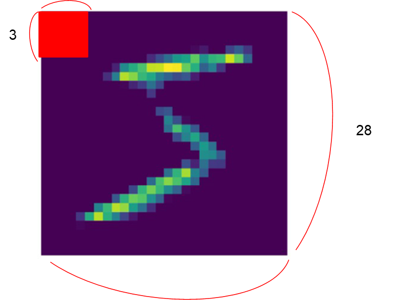

28x28 이미지에 학습이 완료된 3x3 conv 필터가 채널1,2,3 지나감.

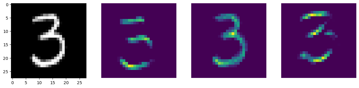
방금 전 과정을 함수로 작성

def draw_feature_maps(n):
    inputs = X_train[n].reshape(-1,28,28,1)
    feature_maps = conv_layer_output.predict(inputs)
    
    fig,ax = plt.subplots(1,4,figsize=(15,5))
    
    ax[0].imshow(inputs[0,:,:,0],cmap='gray');
    for i in range(1,4):
        ax[i].imshow(feature_maps[0,:,:,i-1])
        ax[i].axis('off')
        
plt.show()

# 50번째 숫자 = 3
draw_feature_maps(50)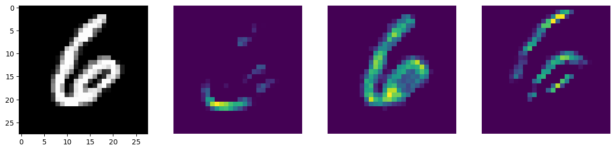

# 13번째 숫자 = 6
draw_feature_maps(13)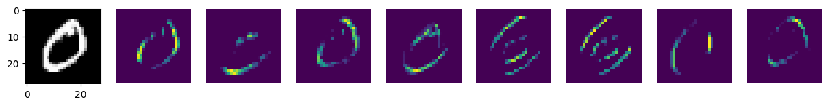

모델 채널 증가시키기

model1 = models.Sequential([
    layers.Conv2D(8,kernel_size=(3,3),strides=(1,1), 
                  padding='same',activation='relu',
                  input_shape=(28,28,1)),
    layers.MaxPool2D(pool_size=(2,2),strides=(2,2)),
    layers.Dropout(0.25),
    layers.Flatten(),
    layers.Dense(1000,activation='relu'),
    layers.Dense(10,activation='softmax')
])

%%time
model1.compile(optimizer='adam',loss='sparse_categorical_crossentropy',
             metrics=['accuracy'])
hist = model1.fit(X_train,y_train,epochs=5, verbose=1,
                validation_data=(X_test,y_test))

Epoch 1/5
1875/1875 [==============================] - 17s 9ms/step - loss: 0.1675 - accuracy: 0.9473 - val_loss: 0.0585 - val_accuracy: 0.9804
Epoch 2/5
1875/1875 [==============================] - 18s 10ms/step - loss: 0.0647 - accuracy: 0.9791 - val_loss: 0.0441 - val_accuracy: 0.9857
Epoch 3/5
1875/1875 [==============================] - 19s 10ms/step - loss: 0.0459 - accuracy: 0.9851 - val_loss: 0.0474 - val_accuracy: 0.9838
Epoch 4/5
1875/1875 [==============================] - 19s 10ms/step - loss: 0.0327 - accuracy: 0.9893 - val_loss: 0.0371 - val_accuracy: 0.9882
Epoch 5/5
1875/1875 [==============================] - 19s 10ms/step - loss: 0.0253 - accuracy: 0.9917 - val_loss: 0.0421 - val_accuracy: 0.9872
CPU times: total: 7min 21s
Wall time: 1min 32s

conv_layer_output = tf.keras.Model(model1.input,model1.layers[0].output)

def draw_feature_maps(n):
    inputs = X_train[n].reshape(-1,28,28,1)
    feature_maps = conv_layer_output.predict(inputs)
    
    fig,ax = plt.subplots(1,9,figsize=(15,5)) #9개 다 그리도록 설정
    
    ax[0].imshow(inputs[0,:,:,0],cmap='gray');
    for i in range(1,9):
        ax[i].imshow(feature_maps[0,:,:,i-1])
        ax[i].axis('off')
        
plt.show()

draw_feature_maps(1) # 0 

draw_feature_maps(13) # 6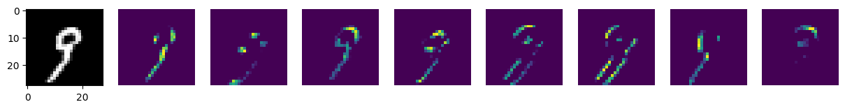

draw_feature_maps(19) # 9

draw_feature_maps(25) #2