
딥러닝
◾Mask Man
얼굴 사진을 이용해 마스크 착용 여부 인식
- data : Kaggle
데이터 준비
zip파일 파이썬 내에서 풀기
import zipfile

content_zip = zipfile.ZipFile("./archive.zip")
content_zip.extractall()

content_zip.close()
colab 사용 시 훨씬 속도 빠르기 때문에 colab으로 이용 추천.
💡colab unzip방법
from google.colab import drive
drive.mount('/content/drive')
# 파일위치 # /content/drive/MyDrive/ds_study/archive.zip
!unzip -qq "/content/drive/MyDrive/ds_study/archive.zip"
ls"./Face Mask Dataset/" Volume in drive C has no label.
Volume Serial Number is 90B1-C6BC
Directory of C:\Users\jjung\Face Mask Dataset
2023-02-09 오후 05:13 <DIR> .
2023-02-09 오후 05:13 <DIR> ..
2023-02-09 오후 05:13 <DIR> Test
2023-02-09 오후 05:13 <DIR> Train
2023-02-09 오후 05:13 <DIR> Validation
0 File(s) 0 bytes
5 Dir(s) 368,433,692,672 bytes free사용 모듈 import
import numpy as np
import pandas as pd
import os
import glob
import matplotlib.pyplot as plt
import seaborn as sns

import tensorflow as tf
from tensorflow.keras import models
from tensorflow.keras.layers import Flatten, Dense, Conv2D, MaxPooling2D, Dropout
from sklearn.model_selection import train_test_split
from sklearn.metrics import classification_report, confusion_matrix
데이터 정리
데이터 읽기
각 폴더의 사진 읽기
ls"./Face Mask Dataset/Train" Volume in drive C has no label.
Volume Serial Number is 90B1-C6BC
Directory of C:\Users\jjung\Face Mask Dataset\Train
2023-02-09 오후 05:13 <DIR> .
2023-02-09 오후 05:13 <DIR> ..
2023-02-09 오후 05:13 <DIR> WithMask
2023-02-09 오후 05:13 <DIR> WithoutMask
0 File(s) 0 bytes
4 Dir(s) 368,424,456,192 bytes freeWithMask / WithoutMask 폴더이름을 라벨로 사용
path = './Face Mask Dataset/'
dataset = {"image_path" : [], "mask_status" : [], "where" : []} #경로, 상태,where:폴더이름

for where in os.listdir(path):
    for status in os.listdir(path + "/" + where):
        for image in glob.glob(path + where + '/'+status + '/' + '*.png'):
            dataset['image_path'].append(image)
            dataset['mask_status'].append(status)
            dataset['where'].append(where)
DataFrame으로 정리
dataset = pd.DataFrame(dataset)
dataset.head()| image_path | mask_status | where | |
|---|---|---|---|
| 0 | ./Face Mask Dataset/Test/WithMask\1163.png | WithMask | Test |
| 1 | ./Face Mask Dataset/Test/WithMask\1174.png | WithMask | Test |
| 2 | ./Face Mask Dataset/Test/WithMask\1175.png | WithMask | Test |
| 3 | ./Face Mask Dataset/Test/WithMask\1203.png | WithMask | Test |
| 4 | ./Face Mask Dataset/Test/WithMask\1361.png | WithMask | Test |
데이터 분포 확인
마스크 착용 분포 확인
print('With Mask : ', dataset.value_counts("mask_status")[0])
print('Without Mask : ', dataset.value_counts("mask_status")[1])

sns.countplot(x=dataset["mask_status"]);
With Mask : 5909
Without Mask : 5883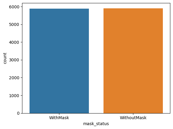
이미지 확인
OpenCV를 활용해 랜덤하게 이미지 확인
import cv2

plt.figure(figsize=(15, 10))
for i in range(9):
    random = np.random.randint(1, len(dataset))
    plt.subplot(3, 3, i+1)
    plt.imshow(cv2.imread(dataset.loc[random, "image_path"]))
    plt.title(dataset.loc[random, "mask_status"], size=15)
    plt.axis('off')
plt.show()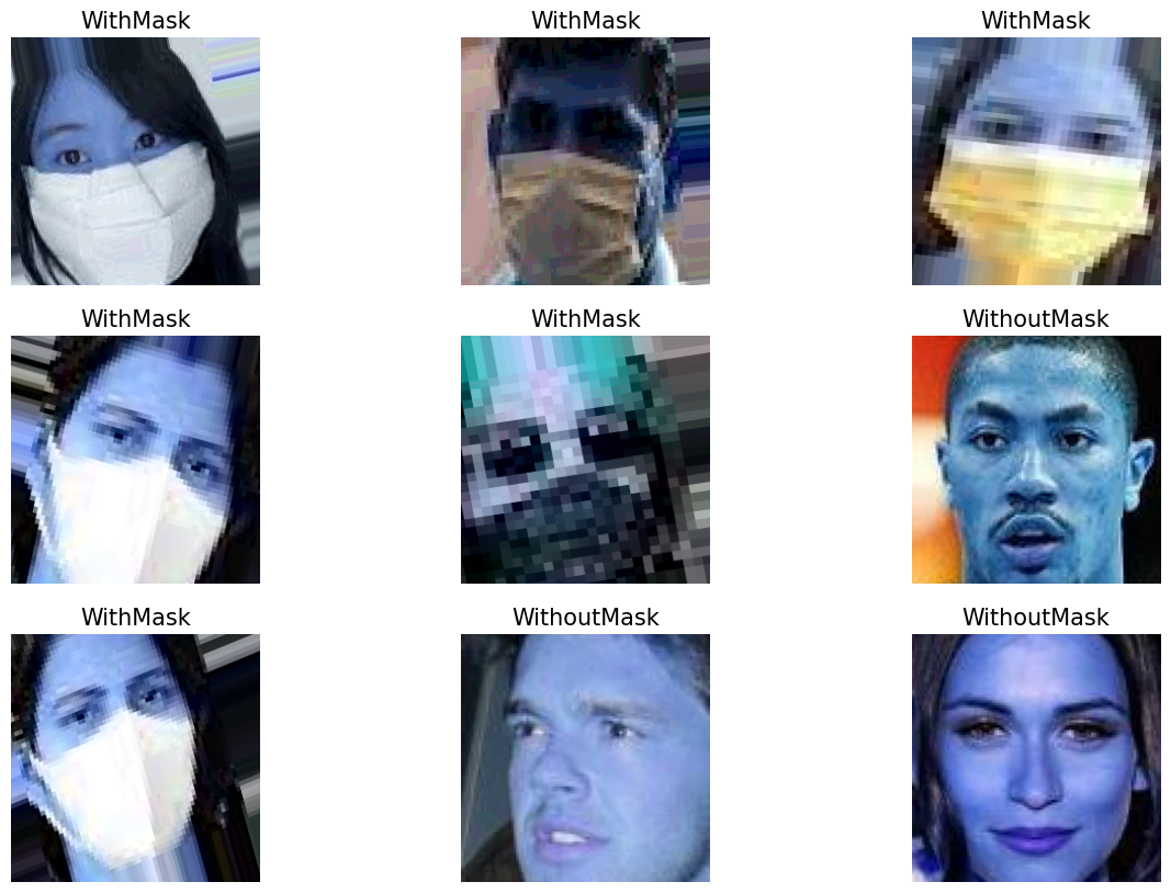
데이터 분리 및 분포 확인
각 폴더에 맞게 데이터 분리
train_df = dataset[dataset['where'] == 'Train']
test_df = dataset[dataset['where'] == 'Test']
valid_df = dataset[dataset['where'] == 'Validation']
# 인덱스 정리 진행
train_df = train_df.reset_index(drop=True)
test_df = test_df.reset_index(drop=True)
valid_df = valid_df.reset_index(drop=True)
train_df.head(2)| image_path | mask_status | where | |
|---|---|---|---|
| 0 | ./Face Mask Dataset/Train/WithMask\10.png | WithMask | Train |
| 1 | ./Face Mask Dataset/Train/WithMask\100.png | WithMask | Train |
Train/Test/Validation 분포 확인
plt.figure(figsize=(15, 5))

plt.subplot(1, 3, 1)
sns.countplot(x=train_df['mask_status'])
plt.title("Training Dataset", size=10)

plt.subplot(1, 3, 2)
sns.countplot(x=test_df['mask_status'])
plt.title("Test Dataset", size=10)

plt.subplot(1, 3, 3)
sns.countplot(x=valid_df['mask_status'])
plt.title("Validation Dataset", size=10)

plt.show()
전처리
이미지 조절
이미지 사이즈 [150 X 150]
data = []
image_size = 150

for i in range(len(train_df)): # 이미지 Grayscale로 변경
    img_array = cv2.imread(train_df['image_path'][i], cv2.IMREAD_GRAYSCALE)

    new_image_array = cv2.resize(img_array, (image_size, image_size))
     #이미지 동일 사이즈 조절

    # 라벨 인코딩
    if train_df['mask_status'][i] == "WithMask":
        data.append([new_image_array, 1])
    else:
        data.append([new_image_array, 0])
Data 쏠림 현상이 있을 수 있으므로 shuffle 해준다.
np.random.shuffle(data)
data[0]
[array([[177, 177, 177, ..., 18, 12, 7],
[177, 177, 177, ..., 18, 12, 8],
[178, 178, 178, ..., 19, 13, 9],
...,
[200, 193, 184, ..., 53, 49, 47],
[200, 191, 180, ..., 50, 47, 45],
[200, 190, 178, ..., 48, 46, 44]], dtype=uint8),
0]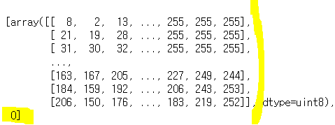
이미지 픽셀값과 라벨 (0)
이미지 확인
fig, ax = plt.subplots(2, 3, figsize=(10, 6))

for row in range(2):
    for col in range(3):
        image_index = row * 100 + col #101번째 ~

        ax[row, col].axis('off')
        ax[row, col].imshow(data[image_index][0], cmap='gray')

        if data[image_index][1] == 0:
            ax[row, col].set_title("Without Mask")
        else:
            ax[row, col].set_title("With Mask")
plt.show()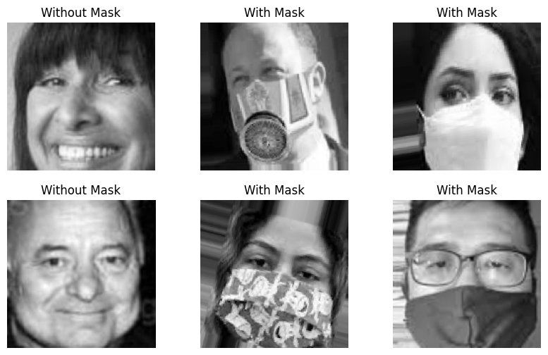
데이터 분리
- X : 이미지 데이터
- y : 라벨(마스크 착용여부)
X = []
y = []

for image, label in data:
    X.append(image)
    y.append(label)

X = np.array(X)
y = np.array(y)

X.shape, y.shape
((10000, 150, 150), (10000,))X_train, X_val, y_train, y_val = train_test_split(X, y, test_size=0.2, random_state=13)모델
LeNet을 기본으로 모델 구현
model = models.Sequential([
                        Conv2D(32, kernel_size=(5, 5), strides=(1, 1), padding='same', activation='relu', input_shape=(150, 150, 1)),
                        MaxPooling2D(pool_size=(2, 2), strides=(2, 2)),
                        Conv2D(64, (2, 2), activation='relu', padding='same'),
                        MaxPooling2D(pool_size=(2, 2)),
                        Dropout(0.25),
                        Flatten(),
                        Dense(1000, activation='relu'),
                        Dense(1, activation='sigmoid')
])model.summary()Model: "sequential"
_________________________________________________________________
Layer (type) Output Shape Param #
=================================================================
conv2d (Conv2D) (None, 150, 150, 32) 832
max_pooling2d (MaxPooling2D (None, 75, 75, 32) 0
)
conv2d_1 (Conv2D) (None, 75, 75, 64) 8256
max_pooling2d_1 (MaxPooling (None, 37, 37, 64) 0
2D)
dropout (Dropout) (None, 37, 37, 64) 0
flatten (Flatten) (None, 87616) 0
dense (Dense) (None, 1000) 87617000
dense_1 (Dense) (None, 1) 1001
=================================================================
Total params: 87,627,089
Trainable params: 87,627,089
Non-trainable params: 0
_________________________________________________________________모델 compile
model.compile(
    optimizer='adam', loss=tf.keras.losses.BinaryCrossentropy(),
    metrics=["accuracy"]
)
모델 학습
X_train = X_train.reshape(len(X_train), X_train.shape[1], X_train.shape[2], 1)
X_val = X_val.reshape(len(X_val), X_val.shape[1], X_val.shape[2], 1)

history = model.fit(X_train, y_train, epochs=4, batch_size=32)
Epoch 1/4
250/250 [==============================] - 158s 632ms/step - loss: 22.6142 - accuracy: 0.8761
Epoch 2/4
250/250 [==============================] - 227s 909ms/step - loss: 0.0844 - accuracy: 0.9712
Epoch 3/4
250/250 [==============================] - 200s 800ms/step - loss: 0.0524 - accuracy: 0.9819
Epoch 4/4
250/250 [==============================] - 206s 822ms/step - loss: 0.0308 - accuracy: 0.9893모델 평가
model.evaluate(X_val, y_val)63/63 [==============================] - 9s 139ms/step - loss: 0.1045 - accuracy: 0.9625
[0.10449627786874771, 0.9624999761581421]prediction = (model.predict(X_val) > 0.5).astype("int32")
print(classification_report(y_val, prediction))
print(confusion_matrix(y_val, prediction)) precision recall f1-score support
0 0.94 0.99 0.96 1013
1 0.99 0.93 0.96 987
accuracy 0.96 2000
macro avg 0.96 0.96 0.96 2000
weighted avg 0.96 0.96 0.96 2000
[[1005 8]
[ 67 920]]잘못 예측한 데이터 확인
wrong_result = []

for n in range(0, len(y_val)):
    if prediction[n] != y_val[n]:
        wrong_result.append(n)

len(wrong_result)75# 잘못 예측한 이미지 출력
import random
samples = random.choices(population=wrong_result, k = 6)
plt.figure(figsize=(14, 12))
for idx, n in enumerate(samples):
plt.subplot(2, 3, idx + 1)
plt.imshow(X_val[n].reshape(150, 150), interpolation="nearest")
plt.title(prediction[n])
plt.axis('off')
plt.show()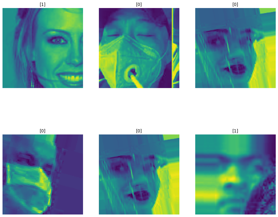

데이터분석 스터디노트🧐✍️