상관 분석
- 두 변수 간의 관계를 살펴보기 위한 방법 중 하나이며, 두 변수가 서로 어떤 관련성을 가지고 있는지 그리고 관련성이 어느 정도인지를 분석하는 방법
ex) 고등학교에서 수학 공부시간과 수학 시험 성적 사이에서는 어떤 관계가 있을까? 수학 공부 시간이 늘어날수록 성적이 올라가는 것일까? 이러한 질문에 대한 답을 찾기 위해 상관 분석을 사용함 - 두 변수 간의 선형적인 관계를 분석함, 따라서 두 변수 간의 관계가 비선형적일 경우 상관 분석을 적용하기 어려움
- 상관 계수는 -1부터 1까지의 값을 가지며 0에 가까울수록 두 변수 간의 상관 관계가 약함을 나타냄
lab12
import seaborn as sns
import pandas as pd

tips=sns.load_dataset('tips')
print(tips)

#corr() : 상관 계수 계산
corr=tips[['total_bill','tip']].corr()
print(corr)
출력
     total_bill   tip     sex smoker   day    time  size
0         16.99  1.01  Female     No   Sun  Dinner     2
1         10.34  1.66    Male     No   Sun  Dinner     3
2         21.01  3.50    Male     No   Sun  Dinner     3
3         23.68  3.31    Male     No   Sun  Dinner     2
4         24.59  3.61  Female     No   Sun  Dinner     4
..          ...   ...     ...    ...   ...     ...   ...
239       29.03  5.92    Male     No   Sat  Dinner     3
240       27.18  2.00  Female    Yes   Sat  Dinner     2
241       22.67  2.00    Male    Yes   Sat  Dinner     2
242       17.82  1.75    Male     No   Sat  Dinner     2
243       18.78  3.00  Female     No  Thur  Dinner     2

[244 rows x 7 columns]
            total_bill       tip
total_bill    1.000000  0.675734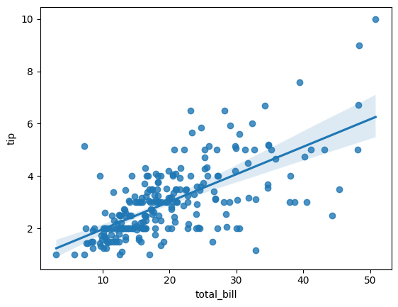
tip 0.675734 1.000000- 두 변수 간의 상관 계수는 약 0.68로 양의 상관 관계가 있다고 해석 됨
- 식사 금액이 높을수록 팁이 많아짐
regplot() 함수를 활용하여 산점도와 회귀선을 동시에 시각화
sns.regplot(x='total_bill',y='tip',data=tips)출력
상관 계수
- 두 변수 간의 관계를 수량화하기 위한 지표
- 대표적으로 피어슨 상관 계수가 있음, -1 부터 1 까지의 범위를 가지며 두 변수 간의 관계를 수량화하여 표현함
import seaborn as sns

# 데이터셋 불러오기
tips=sns.load_dataset('tips')

#total_bill과 tip 간의 피어슨 상관계수 계산하기
corr=tips['total_bill'].corr(tips['tip'],method='pearson')

print('Pearson correlation coefficeint: ',corr)
출력
Pearson correlation coefficeint: 0.6757341092113641- 절댓값이 1에 가까울수록 강한 상관관계를 가짐
- total_bill과 tip 변수 간에 강한 양의 상관관계를 가짐
공분산
- 두 변수 사의 상관 관계의 방향과 강도를 나타내는 지표
# 공분산 실습
covariance=tips['total_bill'].cov(tips['tip'])
print('Covariance between total_bill and tip:',covariance)
출력
Covariance between total_bill and tip: 8.323501629224854- 두 변수는 양의 상관관계를 가지고 있음
산점도
- 두 변수간의 관계를 시각적으로 나타낸 그래프
- x축에는 독립변수, y축에는 종속변수 가 일반적임
- 다중 변수의 관계를 파악하기 위해 선점도 행렬이라는 방법도 존재함
# total_bill과 tip 간의 관계를 산점도 그리기
sns.scatterplot(x='total_bill',y='tip',data=tips)
회귀 직선
- 산점도 상의 두 변수 간 관계를 표현하기 위해 사용되는 선형 함수
- 산점도 상에 분산된 데이터들 사이에서 최대한 데이터를 대표할 수 있는 경향성을 가진 직선을 그리는 것
- 회귀 직선dms y=a+bx 형태로 나타냄, a는 y절편(x=0일 떄의 y r값), b는 기울기(x가 1 증가할 때마다 y가 얼마나 증가하는가) 를 의미
lab13
상관관계 유형 소개
import numpy as np

# 선형 관계 데이터 생성
x_linear=np.linspace(0,10,100)
y_linear=2*x_linear+1

# 비선형 관계 데이터 생성
x_nonlinear=np.linspace(-10,10,100)
y_nonlinear=x_nonlinear**2- linspace() : 시작점과 끝점 사이를 지정한 개수로 일정하게 나눠 배열을 생성함
선형관계
import matplotlib.pyplot as plt

# 선형 관계 시각화
plt.scatter(x_linear,y_linear)
plt.title('Linear Relationship')
plt.xlabel('X')
plt.ylabel('Y')
plt.show()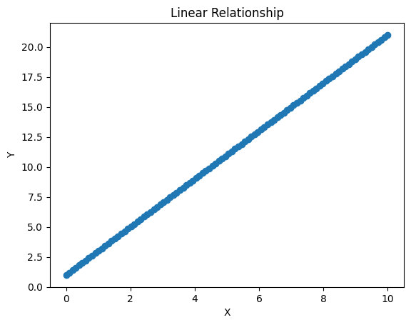
비선형관계
import matplotlib.pyplot as plt

# 비선형 관계 시각화
plt.scatter(x_nonlinear,y_nonlinear)
plt.title('Nonlinear Relationship')
plt.xlabel('X')
plt.ylabel('Y')
plt.show()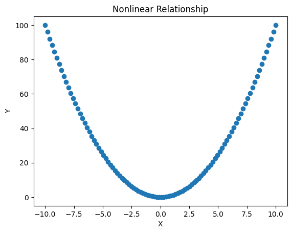
0523
lab01
다중 상관 분석
import seaborn as sns

# titanic  데이터 셋에서 일부 변수 선택
cols=['survived','pclass','age','fare']

# 선택한 변수들을 가지고 새로운 데이터 프레임 생성
df=sns.load_dataset('titanic')[cols].dropna()
print(df)
print('----------------------------------------------------')

# 다중 상관 분석 수행
corr=df.corr()

#결과 출력
print(corr)
출력
     survived  pclass   age     fare
0           0       3  22.0   7.2500
1           1       1  38.0  71.2833
2           1       3  26.0   7.9250
3           1       1  35.0  53.1000
4           0       3  35.0   8.0500
..        ...     ...   ...      ...
885         0       3  39.0  29.1250
886         0       2  27.0  13.0000
887         1       1  19.0  30.0000
889         1       1  26.0  30.0000
890         0       3  32.0   7.7500

[714 rows x 4 columns]
----------------------------------------------------
          survived    pclass       age      fare
survived  1.000000 -0.359653 -0.077221  0.268189
pclass   -0.359653  1.000000 -0.369226 -0.554182
age      -0.077221 -0.369226  1.000000  0.096067
fare      0.268189 -0.554182  0.096067  1.000000
부분 상관 분석
- 두 변수 간의 상관관계에서 다른 변수들의 영향을 제거한 후에 얻어진 상관관계를 계산하는 방법
- 대표적으로 편 상관 계수를 이용함
- 편 상관 계수 :두 변수 간의 상관관계에서 다른 변수 영향을 제거하고 나머지 변수들만으로 계산한 상관계수
시계열 상관 분석
- 시간에 따라 변하는 두 변수 사이의 상관 관계를 평가하는 기술
- 일련의 관측치(ex : 일별 주가, 월별 판매량 등)에서 두 변수 간의 선형 또는 비선형 관계를 파악하는데 사용
- 일반적으로 자기 회귀 모델 및 이동 평균 모델을 사용함
lab02
import pandas as pd
import random
import os

# 랜덤하게 각 주식의 가격 100개의 데이터 생성
# 시계열 데이터는 항상 date형식으로 되어있어야함
dates=pd.date_range(start='2021-01-04',periods=100,freq='D')

# 삼성 전자 주식 데이터
samsung_prices=[random.randint(70000,90000) for _ in range(100)]
samsung_data={'Date':dates,'005930.KS':samsung_prices}
samsung_df=pd.DataFrame(samsung_data)
samsung_df.set_index('Date',inplace=True) # index를 Date로

# LG 전자 주식 데이터
lg_prices=[random.randint(140000,160000) for _ in range(100)]
lg_data={'Date':dates,'066570.KS':lg_prices}
lg_df=pd.DataFrame(lg_data)
lg_df.set_index('Date',inplace=True)

# 두 데이터프레임을 합쳐서 하나의 데이터프레임으로 만들기
df=pd.concat([samsung_df,lg_df],axis=1)
df=df.loc[:,['005930.KS','066570.KS']]
df.columns=['Samsung','LG']

# 폴더가 존재하는지 확인함
# exist_ok:이미 폴더가 생성되어있으면 error가 발생하는데 이를 방지하기 위함
os.makedirs('../data',exist_ok=True)
# csv 파일로 저장
df.to_csv('../data/stock_price.csv')
결과
            Samsung      LG
Date
2021-01-04    83858  156996
2021-01-05    85268  140916
2021-01-06    77379  143397
2021-01-07    74939  149689
2021-01-08    76791  157237
...             ...     ...
2021-04-09    77304  149304
2021-04-10    81356  148745
2021-04-11    87872  150190
2021-04-12    78124  152083
2021-04-13    77708  149614
위의 내용인 Stock_price.csv로 data 폴더에 저장되었음
수익률, 상관 계수 계산
# csv 읽기
df=pd.read_csv('../data/stock_price.csv')
df['Date']=pd.to_datetime(df['Date'])
df.set_index('Date',inplace=True)
print(df)

# 두 종목의 수익률 계산
# 이전의 행값과의 비교를 통해 계산하게 됨
# 이전 값이 없는 2021-01-04 항은 NaN 값이 발생
returns = df.pct_change()
print(returns)

# 수익률 간의 상관 계수 계산
corr_matrix=returns.corr()
print(corr_matrix)
출력
            Samsung      LG
Date
2021-01-04    84442  148737
2021-01-05    71308  155273
2021-01-06    83527  151413
2021-01-07    89668  149309
2021-01-08    76579  143914
...             ...     ...
2021-04-09    82455  152055
2021-04-10    76952  140631
2021-04-11    85507  157621
2021-04-12    83193  152896
2021-04-13    88491  148444

[100 rows x 2 columns]
             Samsung        LG
Date
2021-01-04       NaN       NaN
2021-01-05 -0.155539  0.043943
2021-01-06  0.171355 -0.024859
2021-01-07  0.073521 -0.013896
2021-01-08 -0.145972 -0.036133
...              ...       ...
2021-04-09  0.141467  0.084604
2021-04-10 -0.066739 -0.075131
2021-04-11  0.111173  0.120813
2021-04-12 -0.027062 -0.029977
2021-04-13  0.063683 -0.029118

[100 rows x 2 columns]
          Samsung        LG
Samsung  1.000000 -0.099192
LG -0.099192 1.000000- pct_change() 는 현재 행과 이전 행의 값을 사용하여 변화율을 계산함
히트맵
import seaborn as sns
import matplotlib.pyplot as plt

# 히트맵 그리기
sns.heatmap(corr_matrix,annot=True,cmap='coolwarm')
plt.title('Stock Returns Correlation')
plt.show()
출력
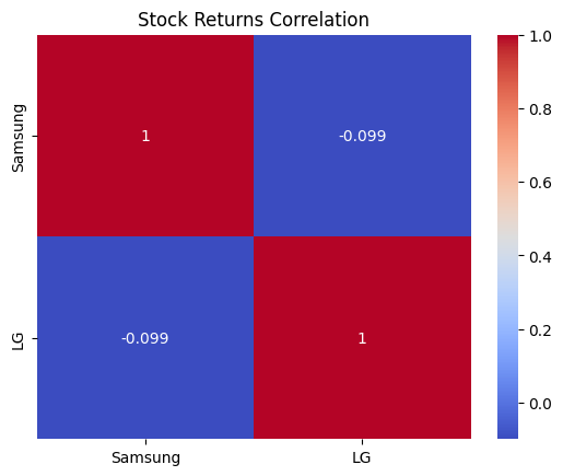
- 상관 계수는 약 -0.072로 나오며 samsung과 lg 주식 가격이 서로 상관 관계가 없다는 것을 의미함
상관 분석의 응용 사례
경제학
ex) 주가와 대통령 선거 결과 사이의 상관 관계 분석, 기업의 매출과 비용의 상관 관계 분석
마케팅
ex) 어떤 제품의 판매량과 광고 비용 간에 어떤 상관 관계가 있는지를 분석하여 광고 비용을 얼마나 투자해야하는지
의학
- 여러 가지 요인이 서로 관련성이 있는지, 질병 예측 및 진단, 치료 효과 분석 등에 이용
기상학
- 기후 변화, 기상 패턴, 날씨 이벤트, 기상 재해 등을 이해하고 예측