Large Concept Models: Language Modeling in a Sentence Representation Space

이번 논문은 meta의 Large Concept Models (LCM) 논문이다. LLM을 대체할지도 모르는 모델이라는 소리까지 들어서 회의적인 시각으로 읽기 시작했는데 어느 정도 그럴듯하다고 느꼈다.

논문의 포인트는 attention을 token 레벨이 아닌 sentence를 embedding화한 concept 단위로 연산하는 것이다.

---

1. Abstract

LLM은 token level에서 처리하지만 이는 다양한 수준의 추상화를 수행하는 사람과 차이가 있다. 따라서 논문은 “concept”이라 이름붙인 higher-level semantic representation에서 수행하는 시도를 한다. concept은 language/modality-agnostic하며 higher level idea/action을 표현한다. 논문은 concept이 sentence에 상응한다고 가정하고 sentence embedding space인 SONAR을 사용한다.

2. Introduction

기존 LLM들은 transformer-based, decoder-only language model이란 공통 구조에 기반하는데, 앞선 tokens이 긴 맥락으로 주어지면 다음 token을 예측하는 식이다. 그러나 이는 사람의 지능이 여러 level의 추상화를 사용하는 것과 차이가 있다. 사람은 top-down 과정으로 먼저 higher level에서 전체적인 구조를 계획하고, 낮은 추상화 level에서 단계별로 detail을 추가한다. LLM도 내재적으로 계층 표현을 배운다고 주장할 수 있지만, explicit hierarchical architecture이 coherent long-form output을 만드는 데 더 좋을 것이다.

그래서 논문은 abstract embedding space에서 hierarchical reasoning을 하는 접근을 제안하며, 이 space는 language/modality에 independent하도록 디자인됐다. 즉 특정 언어가 아닌 순수하게 semantic level을 처리하는 underlying reasoning process를 만드려는 것이다. 연구를 두 추상화 level, subword tokens와 concepts에 한정하며 concept은 abstract atomic idea로 정의한다. concept은 sentence에 상응하며 LLM이 token level인 것과 대비된다.

sentence embedding SONAR (Duquenne et al., 2023b)를 사용하며 text input/output을 200개 언어로 지원하고 speech input을 76개 언어로 지원하고 speech output은 영어를 지원한다.

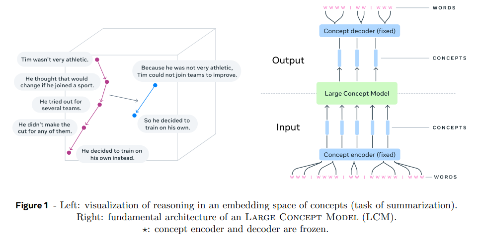
Figure 1 예시 : input을 sentence로 segment > SONAR로 encode해서 sequence of concepts(=sentence embeddings)를 얻고 > LCM이 이걸 처리해서 sequence of concepts를 output > SONAR로 decode해서 sequence of subwords를 구한다.

encoder, decoder는 fixed되어 학습되지 않는다. LCM의 output은 여러 언어나 modality로 decode될 수 있다. 논문은 LCM에 여러 architecture을 탐색해보며 diffusion 변형들을 사용해본다. 추상화 레벨을 paragraph나 small section을 단위로도 실험해본다.

(개인적인 평) 연산 효율이랑 모듈화가 압도적인 장점 같다.
“The LCM can be trained, i.e. acquire knowledge, on all languages and modalities at once, promising scalability in an unbiased way.” SONAR로 encode/decode하는 네트워크만 갈아끼우면 모든 종류의 데이터로 학습 가능한 장점.
인코더/디코더 바꿀 필요도 없다. SONAR가 단일 인코더/디코더로 200개 언어 처리 가능.

3. Method

highly semantic embedding space가 필요한데, xsim/xsim++ 같은 semantic similarity metric에서 최고 성능이며(Chen et al., 2023b), large-scale bitext mining for translation에서 성공적인(Seamless Communication et al., 2023b) SONAR 사용.

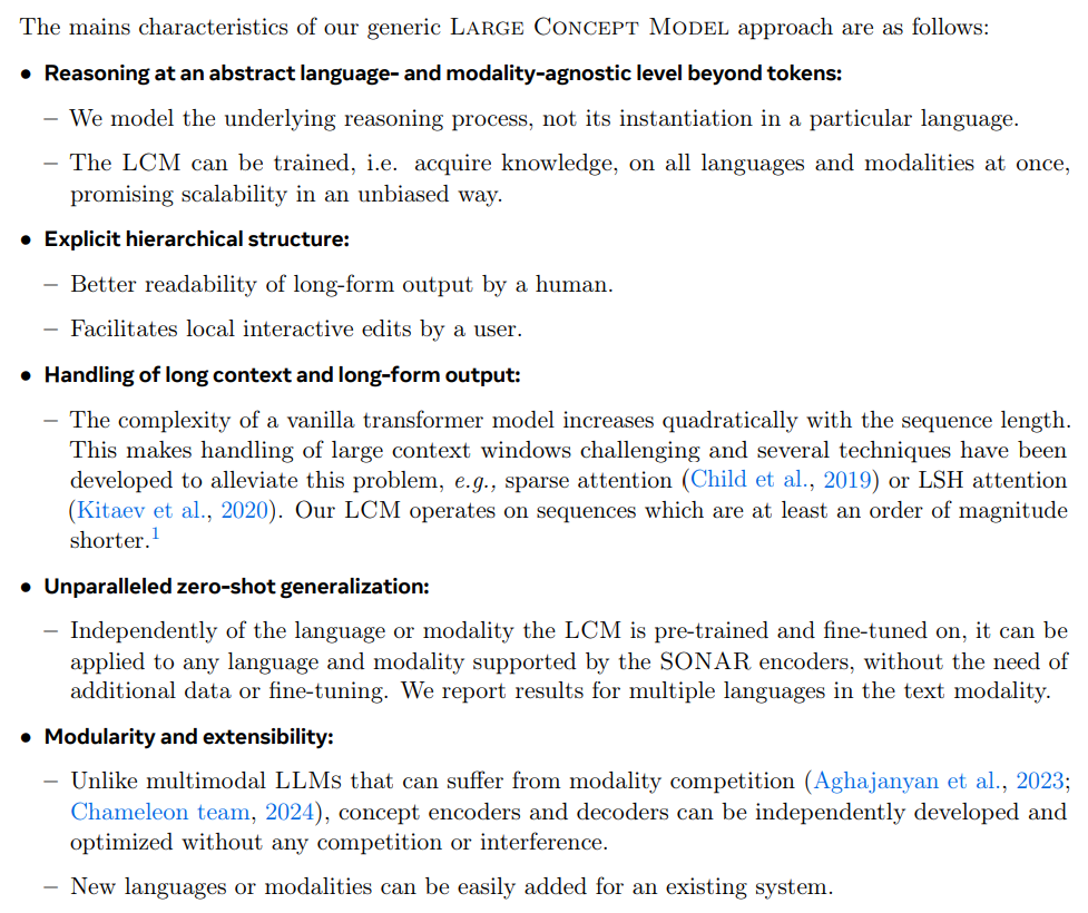
SONAR text embedding space는 encoder/decoder architecture로 학습됐으며 cross-attention 대신 fixed-size bottleneck을 사용했다(즉 인코더가 가변 길이 hidden state를 만드는 게 아니라 입력 문장 하나를 fixed size 벡터로 압축). SONAR training은 3가지 objective, 200개 언어를 영어로 상호 번역하는 machine translation objective, denoising auto-encoding, bottleneck layer에서의 explicit MSE loss를 결합한다. text embedding space를 학습한 후엔 speech modality로 확장하기 위해 teacher-student 방식을 사용한다.

LCM을 학습/평가하려면 raw text datasets을 SONAR embedding sequence로 변환해야한다. 그런데 large text corpora를 다루는 데 몇 가지 어려움이 존재한다. 먼저 text를 sentences로 정확히 segment하는 것이 힘든데, 에러의 존재나 formatting issue, noise 등 때문이다. 그래서 robust automatic text segmentation techniques을 적용한다. 또 어떤 sentences는 아주 길고 복잡할 수 있는데 이는 encoded SONAR embeddings의 퀄리티에 악영향을 끼칠 수 있다. 이 경우는 과학 분야 텍스트에 특히 자주 일어난다.

multilingual data를 다뤄야하므로 많은 language를 다룰 수 있는 2가지 sentence segmenters를 탐색했다.
1. SpaCy segmenter (SpaCy) (Honnibal et al., 2020) : 규칙 기반 다국어 NLP 툴킷, 고자원 언어에 대해 잘 검증됨, 구두점과 대문자에 의존하는 전통적 방식
2. Segment any Text (SaT) (Minixhofer et al., 2023; Frohmann et al., 2024) : 토큰 레벨에서 문장 경계를 예측하는 ML 모델, 구두점/대문자 의존도가 낮아 perturbation에 robust, Split probability threshold 설정에 segment 퀄리티가 dependent

(긴 문장이 인코딩 품질을 저하하니) maximum sentence length 한도 설정(SpaCy Capped, SaT Capped). SpaCy Capped은 구두점 기반 규칙으로 긴 문장 분할, SaT Capped은 분할 확률 추정치를 활용해 최적 분할점 찾기

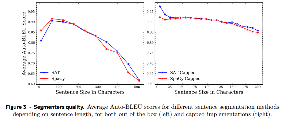
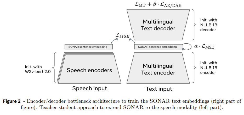
평가는 AutoBLEU 사용, 문장을 SONAR로 encoding, decoding 후 원본 문장과 얼마나 유사한지.
각 segmenter로 documents 가공 후 AUTOBLEU 점수 계산. 문장 길이 200 characters 제한했을 때 SAT Capped가 SpaCy Capped보다 일관적으로 약간 우세. 250 characters를 넘어가면 둘 다 성능 급락. 따라서 LCM training data는 SAT Capped로 준비한다.
(개인적인 평) fixed size vector로 표현할 수 있는 풍부함이 제한적이니 원본 문장이 길수록 내용을 다 담기 힘들어지는 게 당연하다.

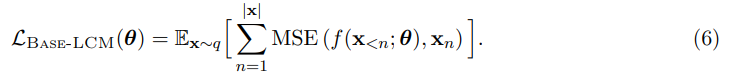
LCM은 continuous sentence embedding을 conditionally 생성해야한다. 이는 기존 LLM이 discrete tokens의 vocabulary에서 확률 분포를 추정하는 방식과 다르다. 간단한 방법은 embedding의 MSE loss를 최소화하도록 transformer를 학습하는 것이지만, 주어진 context가 many plausible, yet semantically different, continuations을 가질 수 있다(즉, 사소한 오차도 의미적으로 큰 차이가 있을 수 있다). 그래서 sentence embedding generation에 diffusion model을 탐색하며, 이후 2 variants를 제시한다. continuous data generation의 또 다른 방식에는 data를 quantize해서 discrete units로 model하는 quantization 방식이 있다.

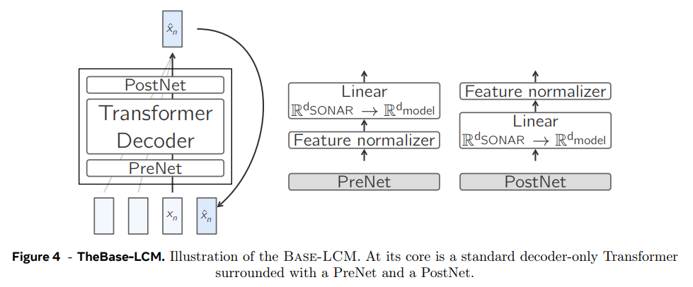
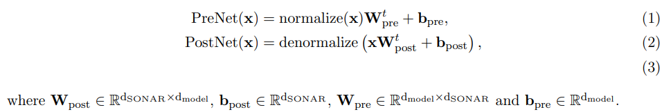
next-concept prediction을 위한 baseline architecture는 과거 concept sequence를 읽고 미래 sequence를 예측하는 standard decoder-only Transformer이다. Base-LCM은 PostNet, PreNet을 가지고 있으며 PreNet은 input SONAR embeddings을 normalize해서 모델의 hidden dimension d_model로 mapping한다.

normalize, denormalize 변환을 학습하기 위해, 다양한 코퍼스와 텍스트 데이터 도메인에서 랜덤 샘플링한 SONAR 벡터 세트로 robust scaler를 학습시킨다. 이 scaler는 중간값(median) 통계를 제거하고 사분위범위(IQR)에 따라 데이터를 스케일링한다.

Base-LCM은 semi-supervised task of next concept prediction으로 학습된다.

inference time에 variable length documents를 생성하기 위해 training documents를 “End of text.” sentence로 suffix한다. 이것도 SONAR로 encode한다. inference 시 2개의 early stopping mechanisms을 사용하는데, 첫째는 generated embedding과 eot의 cosine similarity가 threshold를 넘으면 멈추는 것이고, 두번째는 generated embedding을 직전에 생성된 embedding과 비교해 cosine similarity가 threshold를 넘으면 멈추는 것이다. (둘 모두 threshold를 0.9로 잡았다)

Diffusion-based LCMs은 data distribution q를 근사하는 model distribution $p_\theta$를 배우는 generative latent variable models이다. Base-LCM처럼 diffusion LCM도 한 번에 한 concept씩 auto-regressive하게 생성한다. 따라서 model distribution p는 이전 context가 주어졌을 때(conditioned) 다음 concept를 생성하도록 표현된다. 즉, $p_θ(x_n | x_{<n})$ 형태다.

• Forward process (noising)

timestep t에서 marginal distribution q(x t |x 0 )으로 표현되는 Gaussian diffusion process

reparameterization trick을 적용하면

variance-preserving forward process (Karras et al., 2022)를 사용해서 $(α_t² + σ_t² = 1)$ (즉, 전체 분산을 일정하게 유지한다. $Var(x_t) = Var(x_0)$.)

λ_t는 time step t에서 log signal-to-noise ratio (log-SNR)이다.

noise schedule은 time step t를 log-SNR level로 mapping하는 strictly monotonically decreasing function $f_λ$이다. 즉, $λ_t = f_λ(t)$.

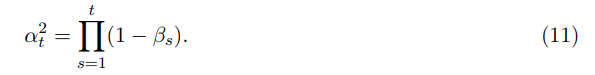
기존엔 forward process를 Gaussian noise를 점진적으로 더하는 discrete time Markov chain으로 간주했고 variance schedule($β_t$)을 했다. variance schedule과 논문의 noise schedule은 식 11과 같이 연관된다.

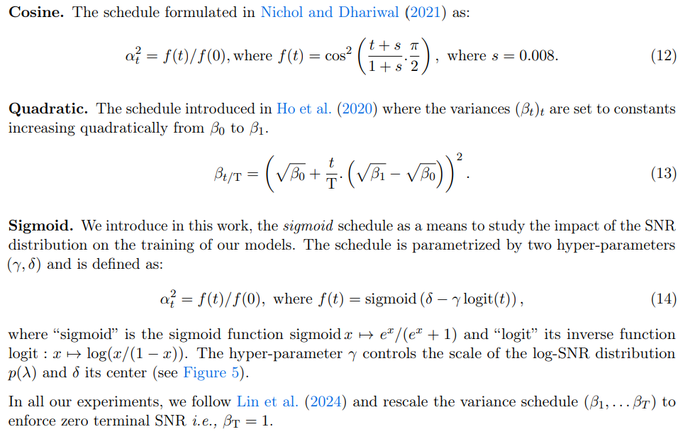
논문에선 3종류의 noise schedules을 고려한다.

• Reverse process (denoising) & objective function

diffusion model $p_θ (x0...1)$의 joint distribution은 reverse process라 불리며 Markov chain with learned Gaussian transitions로 정의된다.

µ, Σ는 predicted statistics이며 Σ는 forward process의 transition과 매칭되는 constant $σ_t^2I$로 설정된다. $µ_θ$는 $x^{t-1}$와 noise approximation model $ϵ_θ$의 선형 조합이다. 이 방법은 ϵ-prediction (Ho et al., 2020; Nichol and Dhariwal, 2021; Nichol et al., 2022)라고 한다.

논문은 $x^0$-prediction을 적용하며, noiseless state를 예측해서 reconstruction loss를 optimize한다.

논문은 default로 simple reconstruction loss (ω(t) = 1, ∀t)를 사용하며 clamped-SNR weighting strategy도 실험한다. 이는 Salimans and Ho (2022)의 truncated-SNR weighting과 Hang et al. (2023)의 min-SNR strategy의 일반화 버전이다.

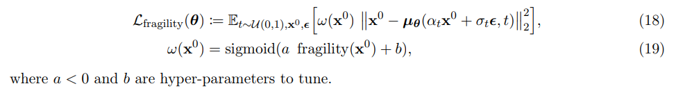
추가로 논문은 sample x0의 quality에 따른 weighting strategy도 고려한다. sample의 fragility score(노이즈 추가 후 복원하기 얼마나 쉬운지)와 연관된 scalar ω(x0) ∈ [0, 1]을 sample weight으로 사용한다. fragile sample은 더 작은 weight을 가져 loss에 덜 기여한다.

• Classifier-free diffusion guidance for the LCM

Classifier-free diffusion guidance (Ho and Salimans, 2022)은 conditional, unconditional diffusion model을 동시에 훈련한다. inference 시 conditional, unconditional score estimates이 식 20과 같이 결합되어 sample quality와 diversity의 trade-off를 달성한다.

y는 conditioning variable이고 논문의 경우 xn을 denoising할 때 sequence of preceding embeddings (x1 , . . . xn−1)이다. hyper parameter γ는 conditional score의 기여를 조절한다. γ = 0이면 unconditional model과 동등하고, γ = 1이면 fully conditional model이다. 실제로는 vision model에선 1보다 큰 값을 사용해 conditioning model의 신호를 증폭한다(guidance).

• Inference

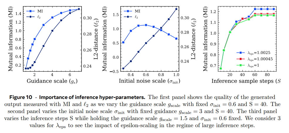
inference 시 reverse process가 적용된다. p(x T) = N (0, I)에서 random noise xT를 sampling하고 score function 방향으로(log-likelihood가 가장 빠르게 증가하는 방향) 반복적으로 step을 취해 denoising된다. 실제로는 x T ∼ N (0, σ2 initI)에서 시작하며 sampled output의 퀄리티가 initial noise scale σinit에 민감했다.

T=100이란 큰 숫자의 discretized timesteps에 모델을 학습했지만 accelerated generation processes (Song et al., 2020)를 사용해 더 적은 수의 S=40 steps에만 생성한다. trailing method of Lu et al. (2022)을 따라 sample steps을 골랐다. 즉 sampled steps (τ1, . . . τS) = round(flip(arange(T, 0, −T/S)))을 따라 generate한다.

image synthesis diffusion models에서 terminal SNR이 0에 근접함에 따라 발생하는 image over-exposure problem을 완화하기 위해 classifier-free guidance rescaling technique of Lin et al. (2024)을 사용한다. (inference에 사용된 guidance scale과 guidance rescale factors는 g_scale과 g_rescale로 표기한다.)

또 diffusion model이 exposure bias problem을 완화하기 위해 inference 시 Ning et al. (2023)을 따라 Epsilon-scaling을 수행한다. 이는 scalar λ_eps로 over-predicted magnitude of error를 scaling down하는, 학습이 필요없는 방법이다.

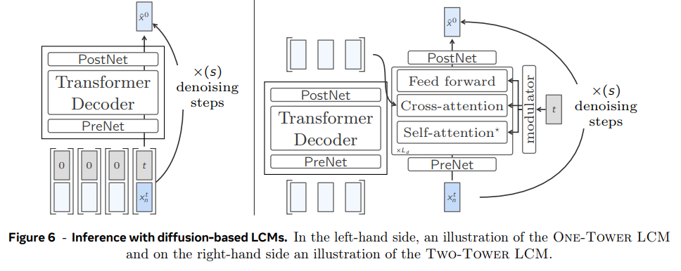
diffusion LCM은 2가지 변형, One-Tower와 Two-Tower 모델이 있다.

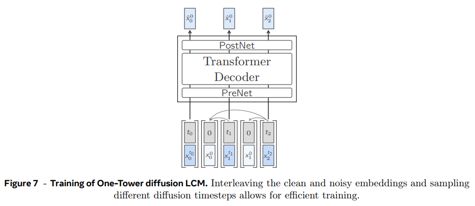
• One-Tower Diffusion LCM

noisy input $x^t_n$이 주어졌을 때 previous clean sentence embeddings $x^0_{<n}$에 condition되어 clean next sentence embedding $x^0_n$을 예측하는 single transformer backbone로 구성된 모델이다. training 중 unconditional training을 위해 특정 확률로 self-attention이 drop될 수 있다. 이는 inference 시 classifier-free guidance를 가능하게 한다.

효율적인 학습을 위해 모델은 document 내의 each and every sentence를 동시에 예측하도록 훈련된다. diffusion 중 모델은 causal multi-head attention layers을 이용해 context 내의 clean sentences를 attend한다. input은 noisy (blue)와 clean (light blue) sentence embeddings을 교차 배치함으로써 준비돼고 clean sentence embeddings (gray arrows)만 attend하도록 attention mask를 적용한다(즉, causal LLM에서 앞쪽 토큰이 뒤쪽 토큰 훔쳐보지못하도록 mask 적용하는 것처럼 학습하려는 noisy sentence가 이전 clean sentence들만 attend하도록 masking).

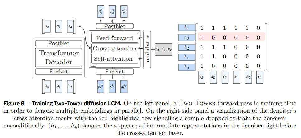
• Two-Tower Diffusion LCM

이 모델은 preceding context encoding을 next embedding diffusion과 분리한다. 첫 부분인 contextualizer은 context vectors x<n을 input으로 받아 causally encode한다. 즉 decoder-only Transformer with self-attention을 적용한다. 그 결과를 두 번째 부분인 denoiser에 전달하고 latent x^1_n ∼ N (0, I)을 반복적으로 denoising해 clean next sentence embedding x^0_n을 예측한다.

denoiser는 Transformer blocks의 stack으로 이루어지며 encoded context와 attend하기 위한 cross-attention block을 가지고 있다. contextualizer, denoiser는 동일한 Transformer hidden dimension d_model을 공유한다. denoiser의 각 block은 adaptive layer norm (AdaLN)으로 조절된다. AdaLN은 현재 timestep t의 embedding에서 channel-wise scale (γ), shift (β), residual gates (α)를 조절한다.

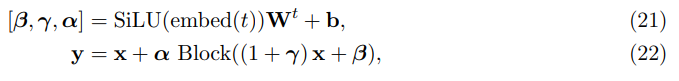
Peebles and Xie (2023)와 Goyal (2017)를 따라 residual block은 W, b를 0으로 설정해 indentity function으로 초기화한다. timestep t는 256-dimensional frequency embedding (Dhariwal and Nichol, 2021; Peebles and Xie, 2023)을 사용해 embed되고 SiLU activation을 가진 two-layer MLP가 뒤따른다. embed 함수는 denoiser의 hidden dimension d_model로 mapping한다. (denoiser의 self-attention layers는 현재 position에만 attend하며, 다시 말해 preceding noised context를 attend하지 않는다. 이는 standard transformer와 일관성을 위해, 그리고 여러 vectors를 한번에 denoising하는 식으로의 확장 가능성을 위해 보존된 것이다.)

training 시엔 unsupervised sequences of embeddings에 next-sentence prediction task로 학습된다. 즉 contextualizer의 causal embeddings가 denoiser에서 한 position만큼 shift되고 cross-attention layers에 causal mask를 사용한다. first position을 예측하기 위해 context vectors 앞에 0 벡터를 추가한다. 여기서도 inference 시 classifier-free guidance scaling를 하려면 conditionally and unconditionally 학습해야하는데, cross-attention mask에서 p_cfg 확률로 random row를 drop하여 해당 position에선 context로 0 벡터만 사용해서 denoise한다.

• Quantized LCM

motivation.
기존에 image나 speech generation에서 continuous data를 생성하는 두 가지 방법으로 diffusion modeling과 data quantization 후 모델링하는 법이 있다. 또 SONAR space에서 continous representation을 다루긴 하지만 여전히 text modality는 이산적이며 모든 가능한 문장은 실제로 연속 분포라기보단 cloud of points 형태다. 또 quantization을 사용하면 randomness/diversity를 조절할 수 있는 temperuatre, top-p, top-k sampling 사용이 가능하다.

따라서 SONAR space를 위한 residual quantizers를 학습시키고 그 discrete units에 Quantized LCM을 만든다. diffusion LCM과 비교를 위해 최대한 비슷한 architecture로 만들었다.

• Quantization of SONAR space

SONAR representation을 이산화하기 위해 Residual Vector Quantization (RVQ; Zeghidour et al. (2021))을 coarse-to-fine quantization 기술로 사용한다. 이는 연속 input embeddings을 learnt codebook 상에서 가장 가까운 entry로 매핑한다. RVQ는 각 iteration마다 additional codebook을 사용해 previous quantizations로부터 residual errors를 반복적으로 quantize한다. iterative k-means clustering of residuals을 수행하는 FAISS implementation (Douze et al., 2024)을 사용한다. 메모리 효율을 위해 beam size 1로 Improved Residual Vector Quantization (IRVQ; Liu et al. (2015))을 사용한다. (즉 FAISS 구현 + IRVQ (beam size=1)) RVQ codebooks은 Common Crawl 데이터셋에서 15M 영어 문장을 codebook 64개, 8192 units per codebook로 학습했다.
(즉 cluster centroid=codebook 하나로 1번 양자화하고 끝내겠다는게 아니라 오차(residual)도 양자화하고, 그것의 오차도 양자화하고…를 64번 반복)

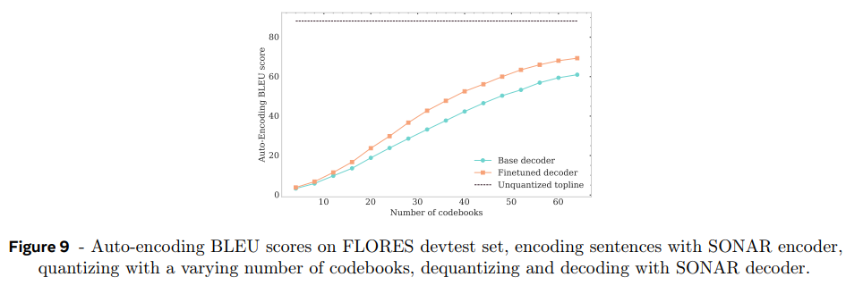
RVQ 특징이 coarse-to-fine, 즉 cumulative approximation을 한다는 것이다. 그래서 codebook을 더 많이 사용할수록 auto-encoding BLEU score가 어떻게 변하는지 관측 가능하다. codebook 수가 증가할수록 BLEU 점수가 70%까지 높아진다.

SONAR decoder를 1.2M 영어 문장를 quantize한 것에 fine-tune했다. decoder가 intermediate codebooks에서 residual representations에 robust하도록 p=0.3 확률로 랜덤하게 codebook number k ∈ [2/3 · n_codebooks, n_codebooks]를 뽑아 k까지만 codebooks을 사용해 quantize했다(즉 덜 세밀하게). Figure 9에서 성능 향상이 보인다.

Quant-LCM architecture의 경우, diffusion LCM과 마찬가지로 left-context sentences에 condition된 coarse-to-fine 생성을 한다. 그러나 denoising task를 diffusion modeling이 아닌 intermediate quantized representations에 기반한 iterative generation of SONAR embeddings으로 간주한다. 먼저 0 벡터인 intermediate representation로 시작해서 predicted residual centroid embeddings를 반복적으로 더해준다. 실험에는 One-Tower architecture을 사용했지만 Two-Tower architecture도 사용할 수 있다. diffusion LCM과 달리 noisy input representation이 intermediate quantized representations로 대체됐고 diffusion timestep embeddings는 codebook index embeddings로 바뀐 것이다.

Discrete targets : Quant-LCM-D
softmax output layer를 가지고 parameterize된 Quant-LCM은 next codebook에서 unit을 예측하도록 학습될 수 있다. parameter 효율을 위해 (n_codebooks · n_units-per-codebook 차원 output을 만들) n_codebooks · n_units-per-codebook unique indices를 discrete target으로 사용하는 게 아니라 codebook index를 모델에 input하고 n_units-per-codebook output dimensions만 예측한다. 학습시엔 diffusion 때와 비슷하게 n_codebooks 이하 codebook index k를 랜덤 sample해서 첫 k-1 codebooks의 centroid embeddings의 cumulative sum을 input으로 사용한다. 그리고 target embedding의 codebook k에서 unit을 target index로 사용해 cross entropy loss를 계산한다. inference 시 반복적으로 next codebook에서 unit을 예측하고, 상응하는 centroid embeddings을(=predicted residual embedding) 얻어서 현재 intermediate representation에 더한다. 마찬가지로 학습 중 left-context conditioning을 drop해서 inference 시 classifier-free guidance가 가능하게 한다. quantized representations을 위한 SONAR decoder를 사용한다.

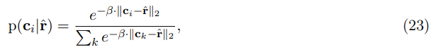
Continous targets : Quant-LCM-C
left-context sentences와 target vector의 intermediate quantized representation에 기반해 continous target SONAR vectors를 예측하는 방식도 탐구했다. MSE로 prediction과 target embeddings를 최소화한다. inference 시 반복적으로 predicted residual r^을 closest centroid embedding에 더하거나 centroid c_i를 다음 분포에서 sample할 수 있다. β는 temperature hyperparameter다.

4. Experiment

• Ablation study

모델들을 Finewebedu dataset (Lozhkov et al., 2024)에 pre-train한다. 크기는 모두 1.6B 파라미터다. 사용 GPU, 모델 아키텍쳐 디테일은 생략. (17p)

pre-training evaluation의 경우 teacher-forcing mode로 LCM inference를 수행하고 metric으로는 L2 distance (ℓ2), Round-trip L2 distance (ℓ2-r), Contrastive accuracy (CA), Paraphrasing (PAR), Mutual information (MI)를 사용한다. 데이터셋으로는 4개 ROC-stories (Mostafazadeh et al., 2016), C4 (Raffel et al., 2019), Wikipedia-en (English Wikipedia dump), Gutenberg의 subset을 이용한다.

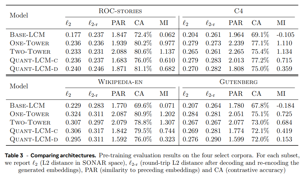
diffusion-based LCM와 Quant-LCM는 objective의 차이에도 불구하고 비슷한 l2, l2-r 점수를 냈다. Base-LCM은 l2-r은 비슷하지만 더 낮은 l2 점수를 냈다. 이는 Base-LCM이 SONAR space에서 plausible modes 중 하나를 sampling하는 대신 average를 생성하기 때문이다(즉 그래서 l2는 낮지만 l2-r은 여전히 높다. CA, MI도 점수가 나쁘다.). CA 점수는 diffusion LCM, QUANT-LCM들이 비슷하지만 MI, PAR 점수는 diffusion 방식이 더 성능이 좋다. 여전히 Quant-LCM이 Base-LCM보다 MI 점수가 더 좋다. 또 Quant-LCM-C가 Quant-LCM-D보다 성능이 좋은데, 논문은 codebook indices의 cross entropy 예측이 MSE objective보다 어려워서 C모델이 left-context vectors의 조합을 더 쉽게 학습한 것이라고 추측한다. diffusion 방식에서 One-Tower, Two-Tower 사이에는 모든 metric/dataset에서 일관적인 차이가 없었다. 전반적으로 SONAR space 상의 next sentence prediction task에서 diffusion 방식이 다른 방법들보다 뚜렷히 좋은 성능을 보였다.

Instruction-tuning evaluation의 경우 Cosmopedia (Ben Allal et al., 2024)의 subset에 instruction-tune해서 평가했다. 비교를 위해 small Llama 모델을 동일한 trainig data (FINEWEB-EDU)에 학습시키고 Cosmopedia에 finetune했다. metric은 ROUGE-L (R-L), Coherence (Coherence)을 사용했다.

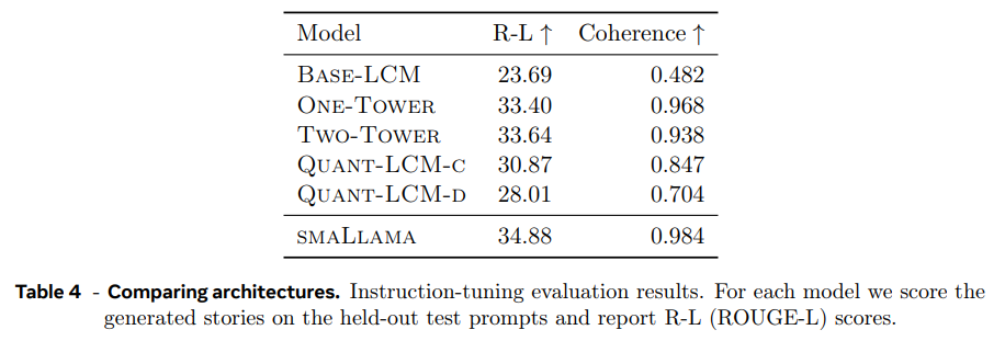
결과는 pretraining evaluation 때와 같으며 Base-LCM보다 다른 모델들이 더 잘하고 diffusion 방식이 quant 방식보다 더 뛰어나다. small Llama가 두 metric 모두에서 LCM보다 뛰어났다. LLM은 fluent output 생성을 잘 하기로 유명하고, diffusion 방식은 small Llama 결과와 동등한 수준이었다.

• Importance of the diffusion inference hyper-parameters

Two-Tower LCM 모델을 사용하여 C4 test split에서 hyperparameter 영향을 분석했다. 설명은 생략.

• Studying the noise schedules

Two-Tower LCM으로 여러 noise schedule을 비교했다.

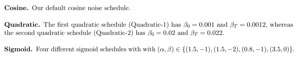
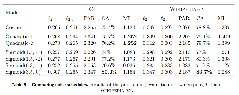
quadratic schedules가 MI score에서 뛰어났고 wide sigmoid schedule (δ, γ) = (3.5, 0)이 CA 점수에서 뛰어났다.

• Studying the loss weighting strategies

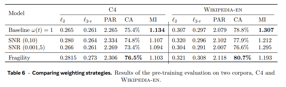
Two-Tower diffusion LCM를 simplified objective ω(t) = 1, ∀t로 학습할 때와 clamped-SNR weighting strategy, fragility-aware weighting strategy를 비교한다. pre-training evaluation metrics 기준 clamped-SNR weighting strategy가 생성된 텍스트의 질을 올리지 않았다. fragility-aware weighting strategy는 CA 점수를 향상시켰다. 이후 실험에는 simplified training objective을 사용했다.

• Inference efficiency of LCMs

Two-Tower LCM과 vanilla LLM의 inference 연산량을 비교한다. LCM은 1.6B, 7B 모델을 사용하고 inference sample steps S = 40으로 inference cost를 추정한다.

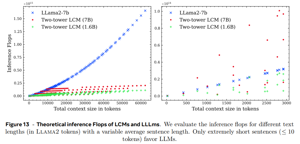
context size를 늘릴 때 LCM이 더 나은 scalability를 보인다. LLM은 짧은 context에서 더 효율적이다.

• Fragility of SONAR space (생략)

• Scaling the model to 7B

Two-Tower diffusion LCM을 7B로도 scaling했다. summarization과 summary expansion(given a summary, create a longer text) task에 실험하며 metric은 Table 8과 같다.

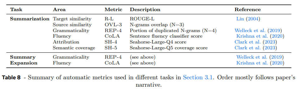
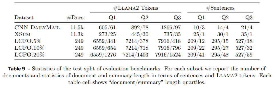
summarization task는 Table 9의 데이터셋을 사용했다. 아주 긴 LCFO는 corpus에서 input document의 5%, 10%, 20% 길이의 abstractive summary를 만들도록 한다.

CNN DailyMail와 XSum 데이터셋은 여러 baseline과 비교한다. encoder-decoder transformer로 T5 (Raffel et al., 2020)를 사용하고, decoder-only LLMs로 LCM과 비슷한 크기의 Gemma-7B, Llama-3.1-8B, Mistral-7B-v0.3를 사용한다. T5는 LCM보다 크기가 더 작아서 target evaluation dataset에 fine-tune하는 식으로 벌충했다. (이래도 되나?)

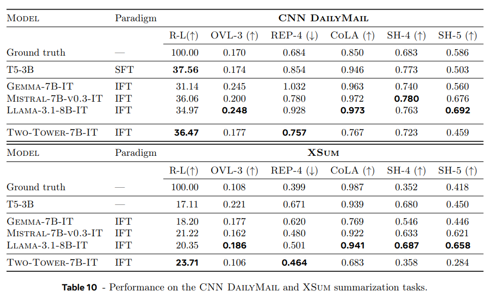
LCM이 Rouge-L 점수에서 specifically tuned LLM (T5-3B)와 경쟁적인 성능을 내고 instruct-finetuned LLMs를 능가한다. LCM이 (원문을 그대로 복사하지 않고) abstractive summaries을 생성해서 OVL-3 점수가 더 낮았고 LLM보다 repetition이 적었다(lower REP-4). 특히 ground truth(인간)와 repetition rate가 비슷했다. CoLA classifier에 따르면 LCM globally less fluent summaries를 생성하지만 사람이 만든 ground truth도 LLM에 비해 낮은 점수를 갖는다. source attribution (SH-4), semantic coverage (SH-5)도 비슷한 경향을 보이는데 model-based metrics가 LLM generated content로 편향되어 있기 때문으로 추측된다.

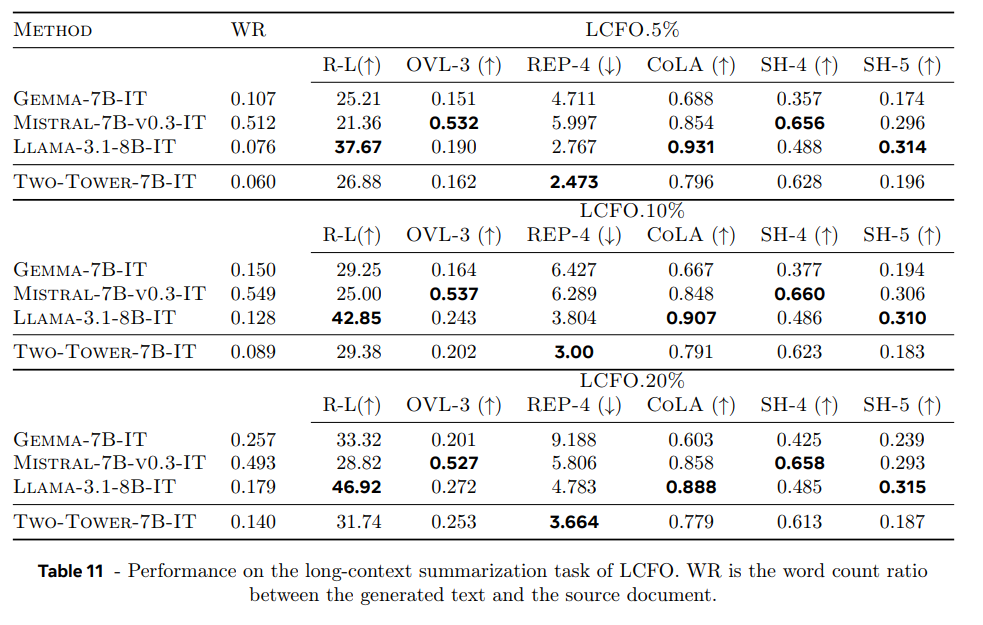
LCM은 학습 중 긴 documents를 한정된 개수만 봤지만 Long-context summarization를 잘한다. Rouge-L 점수에서 5%, 10%일 때 Mistral-7B-v0.3-IT and Gemma-7B-IT를 능가하고 20%일 때 Gemma-7B-IT와 비슷하다.

• Summary Expansion

CNN DailyMail, XSum 데이터셋에서 summary를 input으로 받아 long document를 생성한다. baseline, metric은 동일하다.

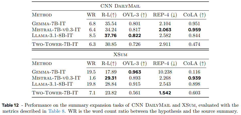
데이터셋 간 생성량이 달랐는데, CNN DailyMail은 모델들이 input보다 6~8배 긴 output을 생성했고 XSum에선 Gemma-7B-IT와 Llama-3.1-8B-IT는 20배나 긴 output을 생성했지만 LCM은 CNN DailyMail과 비슷한 배율로 생성했고, Mistral-7B-v0.3-IT는 길게 생성하는 데 실패했다.

summarization task와 달리 LLM이 LCM보다 더 높은 Rouge-L 점수를 받는다(=원본 문서 내용을 더 많이 재현). 그러나 LLM과 달리 LCM은 original document와 다른 문장을 생성한다. 이는 LCM이 embedding을 생성하고 그게 decoder로 translate되기 때문에 내용을 paraphrase하기 때문으로 추측된다. 그러나 CoLA 결과는 이 과정이 lower fluency를 야기함을 보인다(즉 문법이 나빠진다).

• Zero-shot generalization performance

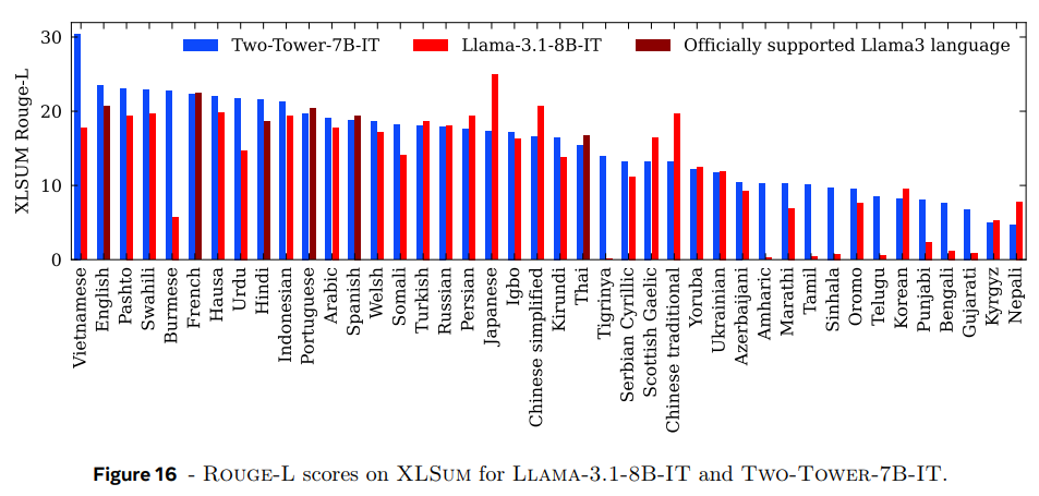
지금껏 실험은 영어 text로 수행됐는데, 이제 LCM이 다른 언어에 zero-shot할 수 있는지 탐구한다. 45개의 언어를 다루는 large scale multilingual abstractive news summarization benchmark인 XLSum (Hasan et al., 2021) 데이터셋을 사용한다. 8개 언어를 지원하는 Llama-3.1-8B-IT와 성능을 비교한다. Figure 16의 결과를 보면 LCM이 영어와 Llama가 지원하는 6개 언어(SONAR가 지원 안하는 언어라 2개는 빠진듯)에서 Llama보다 성능이 좋았다. LCM은 다른 많은 언어에도 일반화가 잘 됐다. 이는 한 번도 본 적 없는 언어에 LCM이 뛰어난 zero-shot generalization 성능을 지녔음을 보여준다.

• Exploring explicit planning

긴 text를 작성할 때 먼저 전체 구조를 짜는 게 중요하다. LCM도 coherent 생성을 위해 planning 능력이 필요하다. 논문은 prior context가 주어졌을 때 다음에 무엇이 생성되어야할지 high-level overview를 생성하는 complementary planning model을 제안한다. plan은 paragraph처럼 복수의 concepts을 다룰 수 있다. LCM은 다음 sequence를 생성할 때 이 plan에 condition된다.

LCM은 paragraph break 같은 주제 전환점을 표현하는 break concept을 기준으로 sequence of concepts를 auto-regressively 예측하고, break concept이 생기면 large planning model (LPM)이 plan을 생성해 LCM에 다음 sequence 생성을 위해 condition시킨다. LCM은 prior concepts와 proposed plan 모두에 condition되어 생성을 이어간다.

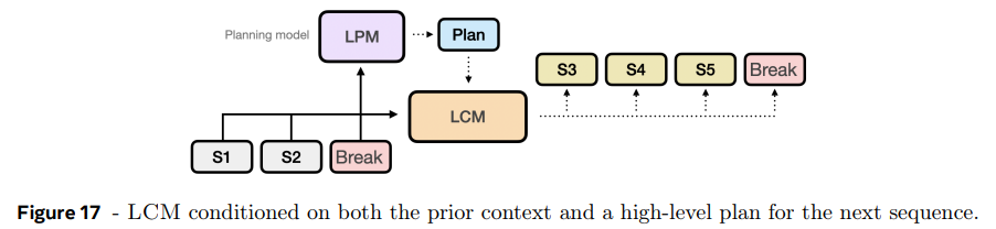
구현을 단순화해 LCM이 break concepts와 plan을 모두 생성하도록 multitask setting으로 학습시키고, paragraph 같은 multiple concepts에 걸친 plan 대신 single concept 수준으로 계획한다. 이 simplified multitask approach를 Large Planning Concept Model (LPCM)이라 부른다.

ablation study를 위해 baseline으로 One-Tower LCM을 사용했다. 그리고 LPCM을 baseline과 같은 수의 파라미터, 데이터셋, step 수로 학습시켰다.

break concepts을 표현하기 위해 먼저 Segment Any Text (Frohmann et al., 2024) paragraph splitting API로 데이터를 문단으로 segment했다. 이때 한 문단이 10 문장 이하도록 했고 연속된 작은 문단은 합쳐줬다. plan concepts을 표현하기 위해 Llama-3.1-8B-IT를 사용해 각 preceding segmented paragraph에 대해 synthetic high-level topic description를 생성했다.

coherence를 main metric으로 사용했다. Llama-3.1-8B-IT를 사용해 output의 coherence score을 [0, 5] 범위로 측정한다. 이 방식의 유효성을 검증하기 위해 Jwalapuram et al. (2022)의 human judgements dataset에 평가해서 사람과 일치함을 확인했다.

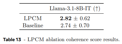
Cosmopedia (Ben Allal et al., 2024) subset에의 결과이며 LPCM이 baseline One-Tower LCM보다 높은 coherence score을 달성한다. 이는 LPCM이 plan concepts을 예측하여 LCM보다 더 coherent output을 생산함을 의미한다.

5. Related Work

Multilingual sentence representations
-learning general sentence representations, leveraging dual encoder architectures (Guo et al., 2018; Reimers and Gurevych, 2019; Ni et al., 2021), encode the source and target into a common embedding space, and use a distance-based metric to create an alignment loss that approximate semantically identical sentences.
-extended to leverage multilingual data to create general, aligned embedding spaces across languages (Feng et al., 2020; Janeiro et al., 2024; Sturua et al., 2024)

• leveraged the contrastive loss to align translations across languages (Feng et al., 2020; Yang et al., 2019)
  -Recent approaches explore using data from other tasks, besides translation data, to increase the generality of the sentence representations (Wang et al., 2024b; Mohr et al., 2024)
  -change their embeddings per task, either with task-specific prompts (Wang et al., 2024b; Su et al., 2022; Lee et al., 2024b) or with task-specific parameters (Sturua et al., 2024).
  -LASER (Artetxe and Schwenk, 2019), and SONAR (Duquenne et al., 2023b) leverage an encoder-decoder architecture

LLM based sentence representation
-Wang et al. (2024a) proposed extracting text embeddings from the last token of LLMs fine-tuned with instructions on contrastive data.

• Lee et al. (2024a) improved text embedding capabilities of fine-tuned LLMs by removing the causal attention mask and applying extra nonlinear layers before pooling the token embeddings

Sentence embeddings for language modeling
-For text completion, Ippolito et al. (2020) proposed a sentence-level language model operating by choosing the next sentence from a finite set of candidates.
-INSET architecture (Huang et al., 2020) solves the sentence infilling task by combining a denoising autoencoder that encodes sentences into fixed-size vectors and decodes them back and a bidirectional transformer that predicts the embedding of a missing sentence.
-Marfurt and Henderson (2021) and Cornille et al. (2024) used predicted next sentence embeddings in a fully generative setting, for summarization and generic language modeling, respectively. However, their architectures considered sentence-level connections only as an addition to the token-level connections across sentences, not as their replacement.
-An et al. (2024), the SentenceVAE architecture performs language modeling on the sentence level using a sentence encoder to prepare the inputs and a sentence decoder to produce the outputs. However, its input and output embedding spaces are not tied

Language modeling with diffusion
-PLANNER architecture (Zhang et al., 2023) consists of a variational autoencoder for paragraphs and a diffusion model trained to predict latent autoencoder representations conditional on the textual context or on the class label.
-Lovelace et al. (2024) augmented a decoder-only language model with an encoded semantic proposal of the continuation text, with an easily guidable diffusion model predicting the embedding of the next proposal.
-TEncDM model (Shabalin et al., 2024) performs diffusion in the space of contextual token embeddings which are then decoded non-autoregressively.

기존 연구들은 token-level input/output에 의존하거나 arbitrary length text를 생성하지 않는다. LCM은 highly semantic, reconstructable sentence representation space로 구현된 최초의 generative language model이다.

6. Limitations

• Choice of the embedding space
  -SONAR embedding은 multilingual/multimodal representation이라 선택됐지만 학습된 bitext machine translation 데이터는 짧은 문장으로 이루어졌다.
  -SONAR는 local geometry를 학습하지만 next sentence prediction은 globally 잘 작동하기를 요구한다.
  -link/referecne/code 등이 SONAR training data나 흔한 LLM pre-training text와 분포가 맞지 않아 LCM은 그런 내용을 포함한 문장 예측이 어렵다.
  -Frozen encoder 방식에 trade-off가 있다. 여러 언어/모달리티 표현 가능해서 데이터 효율적이지만 end-to-end 학습이 아니라 LCM에 최적화되진 않는다. 하지만 동시에 end-to-end 학습이 결과 space가 여러 언어/모달리티에서 좋은 semantic representation을 가질지 보장할 수 없다.

• Concept granularity(세분화) 한계
  -concept=문장으로 정의됐지만 가능한 next sentence 범위가 매우 넓다. 문장 길이도 variale length라 fixed size embedding으로 한계가 있다. Text splitting, 하나의 sentence를 여러 embeddings으로 매핑하는 one-to-many mapping이 향후 연구 방향이다.
  -document의 각 문장은 거의 unique하고 반복되지 않는다. 즉 data가 saprse해서 일반화 능력이 제약된다.
  -이 단점들은 text를 여러 source에서 공통적인 새로운 conceptual units으로 분할하는 방식으로 완화할 수 있다.

• Continuous versus discrete
  -문장이 연속 벡터로 표현되지만 결국 이산적 조합이라 diffusion에 한계가 있다.
  -next token prediction에서 softmax output에 cross entropy loss 적용하는 방식이 여러 downstream task에서 중요한데 continous diffusion은 이 방식을 사용할 수 없다.
  -Quant-LCM이 discrete 방식을 다룰 수 있지만 SONAR가 효과적으로 양자화되게 학습된 게 아니라 RVQ units combinations 수가 지수적으로 폭발한다.
  -결국 새로운 representation space가 필요하다.

---

7. 개인적인 평

나는 사람이 higher level에서 전체적인 계획을 설립한다는 게 CoT 레벨이라고 봐서 이걸 concept level로 두는 건 미스매치라고 생각한다.

또 순수 semantic level을 다루겠다고 하는데, 이거도 이미 LLM이 내재적으로 하는 거라고 본다. 물론 논문은 이걸 사람이 다룰 수 있는 명시적 레벨을 설정해서 더 효과적으로 만든다는 점이 장점이다.

기존의 token 단위 의미 처리를 concept 단위 의미 처리로 확장한 것이 핵심이다. 즉 하나의 임베딩이 표현하는 의미가 더 풍부해져서 연산 효율이 압도적으로 좋아질 듯하다. (바닐라 트랜스포머는 연산량 길이에 quadartically하게 늘어나니)

임베딩의 표현력이 더 풍부해지니 concept 벡터 하나가 (언어로 표현되지 않는 추상적) schema에 대응할 수 있다. 또 원래 concept을 표현하려면 토큰 여러개를 합쳐야했는데 여기선 하나로 가능.

그러나 한계에서도 지적했다시피 concept=문장으로 두는 가정이 너무나 임의적이고 naive하다. concept=문장이 나쁜 choice는 아닌데 최선은 아니다. 한계도 있다.

그러나 단순히 concept 단위를 문장에서 문단으로 변화시킨들 같은 문제가 반복될 것이다. 차원이 너무 커져서 처리도 복잡해질 수 있다. 즉, 문제는 LCM에 사용할 fixed size embedding이 필요한데, 그걸 sentence로 고정하니 문제고, 그렇다고 token은 너무 단위가 작고, paragraph는 크다.
-> 그 사이에서 네트워크가 concept unit 크기(=receptive field)를 동적으로 조절할 수 없나?
네트워크에 전체 text corpus를 (토큰 단위로) 넣으면 알아서 unit 단위로 (합치고) 분할해주도록. unit마다 ‘정보량’이 비슷하고, ‘정보량’이 일정 범위에 들어오도록(왜냐면 fixed size embedding은 특정 최대 크기의 정보까지만 압축할 수 있을테니까. 정보량 기준은 perplexity 사용하면 될듯?) 이때 각 unit 간 정보 중복도(redundancy, mutual information으로 측정?)를 설정해서 실험할 수도 있을 것이다. independent, 30% 겹침, 50% 겹침 등등. 굳이 redundancy를 고려하는 이유는 concept들이 continuous space에서 그나마 dense하게 만들수 없을까 싶어서다.
여기서 최적 크기를 선택하도록 강화학습을 끼워넣을 수 있을지도 모르겠다.
애초에 사람이 감각을 인식할 때도 시청각에선 자극이 파동으로 들어오는데 거기서 뇌가 알아서 의미 단위(물건의 윤곽이라던가, 단어의 음절이라던가)를 구분해서 그걸 unit으로 처리한다. 즉 unit을 segment하는 게 동적으로 가능해야한다.

또 continuous embedding 예측으로 diffusion 사용을 선택한 게 훌륭하다. diffusion의 문제점이 디퓨전하는 크기를 어떻게 조작하느냐인데 여기선 애초에 fixed embedding size를 diffusion하고 context에 따라 autoregressive하게 concept을 생성하니 굉장히 깔끔하게 디퓨전을 사용한다. LLM은 discrete한 vocabulary 내에서 투표시키는 방식이라 output하는 의미가 선택지를 고르는 방식인데 LCM은 의미로 continuous vector를 만드는거라 이게 직관적으로 더 옳은 방식 같다.

사소하게 흥미로웠던 테크닉. Round-trip L2 distance로 reencoding해서 오차 측정하는것으로 OOD 정도 파악.

궁금한 점
1. 현재 구현 안에서 개개 토큰과 문장의 관계는 어떻게 됄까? "비행기가 날다"란 문장과 "비행기", "날다"의 임베딩은 어떻게 연관되나? 그리고 비슷한 문장의 유사도가 높나? sonar 논문을 읽어봐야. (즉 어떤 concept과 그 concept을 구성하는 concept(들) 사이 관계가 궁금하다)
2. concept level에서 prompting이 가능할까? 그러니까 concept output에 "먹고 싶은 음식에 대해 문장을 3단어로 만들자" 이렇게 하면 sonar > token으로 디코딩할 때 그대로 "먹고 싶은 음식에 대해 문장을 5단어로 만들자"와 의미가 비슷한 문장이 나올까 아니면 "햄버거를 먹고 싶다"가 나올까? SONAR 디코더가 translation 기반이라 instruction following보다는 content generation에 특화되어 있을 것 같긴 하다.