
프로젝트 개요

이번 프로젝트는 통계청에서 주관하는 통계데이터 인공지능 활용대회에 참여한 결과물이다. 자연어 기반의 통계데이터를 인공지능으로 자동 분류하는 기계학습 모델을 발굴하는 대회이다. 처음으로 제대로 참여해본 대회라 거의 제로 베이스로 시작하여 부족한 점이 매우 많았고 학습이 잘 돌아가게 만드는 것이나 결과물 제출 형식을 만들어내는 것만으로도 많은 노력이 필요했다. 조잡한 결과물이지만 전체적으로 리뷰하며 부족했던 점들과 보완해야할 점들을 정리해보는 시간을 가지고자 한다.
환경 설정 및 라이브러리 불러오기
한국어 정보처리 패키지인 konlpy를 설치하고 TPU 연산을 위한 설정을 해준다.
!pip install konlpy

%tensorflow_version 2.x
import tensorflow as tf
print("Tensorflow version " + tf.__version__)

try:
  tpu = tf.distribute.cluster_resolver.TPUClusterResolver()  # TPU detection
  print('Running on TPU ', tpu.cluster_spec().as_dict()['worker'])
except ValueError:
  raise BaseException('ERROR: Not connected to a TPU runtime; please see the previous cell in this notebook for instructions!')

tf.config.experimental_connect_to_cluster(tpu)
tf.tpu.experimental.initialize_tpu_system(tpu)
tpu_strategy = tf.distribute.experimental.TPUStrategy(tpu)
필요한 라이브러리들을 불러온다.
from tensorflow.keras.preprocessing.sequence import pad_sequences
from tensorflow.keras.callbacks import EarlyStopping, ModelCheckpoint
from tensorflow.keras import layers
from tensorflow.keras.models import Sequential
from tensorflow.keras.layers import Dense
from tensorflow.keras.preprocessing.text import Tokenizer
from tensorflow.keras import regularizers
from keras.layers import Embedding
from sklearn.model_selection import train_test_split
import matplotlib.pyplot as plt
import numpy as np
import pandas as pd
from tqdm import tqdm
import tensorflow as tf
from konlpy.tag import Okt
import os
import json
import random
import pickle
import re
SEED_NUM = 42
tf.random.set_seed(SEED_NUM)
데이터 불러오기
train 데이터와 submit 데이터를 불러온다. train셋 대회측에서 제공한 전국사업체조사 샘플데이터로 7개의 열과 100만개의 행으로 이루어져 있다. 열은 AI_id, digit_1(대분류), digit_2(중분류), digit_3(소분류), text_obj(무엇을 가지고), text_mthd(어떤 방법으로), text_deal(생산,제공하였는가)로 이루어져있다.
데이터의 특성상 대분류 → 중분류 → 소분류로 내려가는 하위구조이기에 digit_3(소분류)만 예측하면 나머지는 자동으로 할당해줄 수 있다. 따라서 모델의 target을 digit_3로 잡고 학습을 진행하면 된다. 제출용 submit data는 10만개의 text_obj, text_mthd, text_deal이 제공되어 있다.
대부분의 text 길이가 길지 않고 문장형식으로 보기 어렵기에 3개의 열을 하나로 합쳐 학습에 활용하였다. 이는 NA가 있는 행을 없애는 효과도 같이 나타난다.
raw_data = pd.read_table('/content/drive/MyDrive/StatisticCompetition/train.txt',sep='|', encoding='cp949')
submit_data = pd.read_table('/content/drive/MyDrive/StatisticCompetition/2. 모델개발용자료.txt',sep='|', encoding='cp949')

def preprocess(raw_data):  # 텍스트를 하나로 합친다.
    data = raw_data.copy()
    data = data.replace(np.nan, '', regex=True)        # NA가 존재하는 행 없애는 용도
    data = data.rename(columns={'digit_3':'label'})    # 타깃 변수명 변경
    data['document'] = data['text_obj'] + ' ' + data['text_mthd'] + ' ' + data['text_deal']
    data = data.drop(['text_mthd', 'text_deal', 'text_obj', 'AI_id'], axis=1)

    data = data.dropna()
    data = data.reset_index(drop=True)

    return data

data = preprocess(raw_data)
submit = preprocess(submit_data)
digit_1 digit_2 label document
0 S 95 952 카센터에서 자동차부분정비 타이어오일교환
1 G 47 472 상점내에서 일반인을 대상으로 채소.과일판매
2 G 46 467 절단하여사업체에도매 공업용고무를가지고 합성고무도매
3 G 47 475 영업점에서 일반소비자에게 열쇠잠금장치
4 Q 87 872 어린이집 보호자의 위탁을 받아 취학전아동보육
... ... ... ... ...
999995 C 13 134 제품입고 워싱 청바지워싱
999996 F 42 424 현장에서 고객의요청에의해 실내인테리어
999997 G 47 474 영업점에서 일반소비자에게 여성의류 판매
999998 P 85 856 사업장에서 일반고객을대상으로 필라테스
999999 I 56 561 사업장에서 접객시설을 갖추고 한식(미역구)판매
1000000 rows × 4 columns간단한 EDA
label 별로 몇 개의 데이터를 가지고 있는지 확인해 보았다. 12만개가 넘개 있는 label도 있고 반대로 1개 밖에 없는 label도 있었다. label이 총 225개 있는데 클래스 불균형 문제를 가지고 있음을 확인하였다. 따라서 이를 해결해주어야 한다. 이 상태로 학습을 진행할 경우 train accuracy는 매우 높게 나오는데 새로운 데이터셋에서 낮게 나오는 문제가 발생한다.
극단적인 예로, 1과 0을 분류하는 문제에서 1이 97개 0이 3개인 데이터가 있을 때 모든 결과를 1로 예측하는 모델은 이 경우 97%의 정확도를 가지지만 새로운 데이터가 5:5 비율을 가지고 있을 경우 정확도가 50% 밖에 나오지 않는다.
import seaborn as sns
sns.set(rc = {'figure.figsize':(20,15)})
sns.countplot(data['label'])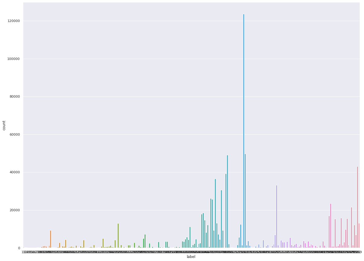
데이터 전처리
1. Easy Data Augmentation(EDA)
앞의 클래스 불균형 문제를 해결해주기 위해 EDA기법을 활용하여 데이터를 증강해주었다. label의 갯수가 500개 이하인 데이터에 대해 각각 위치를 바꾸거나, 새로운 단어를 삽입하거나, 삭제하거나, 대체하여 원본 데이터와 최대한 비슷한 새로운 데이터를 생성해주었다.
총 74,300개의 새로운 데이터를 만들었다. 하지만 한글의 특성 상 이런 과정이 의미가 변형되어버리는 경우가 생기기에 제한적으로 사용되야 함은 인지해야한다. 물론 이번 프로젝트의 경우 성능 향상이 있었기에 활용하였다! wordnet.pickle은 상기 링크에서 다운로드 받을 수 있다.
wordnet = {}
with open("/content/drive/MyDrive/StatisticCompetition/wordnet.pickle", "rb") as f:
	wordnet = pickle.load(f)

########################################################################
# Synonym replacement
# Replace n words in the sentence with synonyms from wordnet
########################################################################
def synonym_replacement(words, n):
	new_words = words.copy()
	random_word_list = list(set([word for word in words]))
	random.shuffle(random_word_list)
	num_replaced = 0
	for random_word in random_word_list:
		synonyms = get_synonyms(random_word)
		if len(synonyms) >= 1:
			synonym = random.choice(list(synonyms))
			new_words = [synonym if word == random_word else word for word in new_words]
			num_replaced += 1
		if num_replaced >= n:
			break

	if len(new_words) != 0:
		sentence = ' '.join(new_words)
		new_words = sentence.split(" ")

	else:
		new_words = ""

	return new_words

def get_synonyms(word):
	synomyms = []

	try:
		for syn in wordnet[word]:
			for s in syn:
				synomyms.append(s)
	except:
		pass

	return synomyms

########################################################################
# Random deletion
# Randomly delete words from the sentence with probability p
########################################################################
def random_deletion(words, p):
	if len(words) == 1:
		return words

	new_words = []
	for word in words:
		r = random.uniform(0, 1)
		if r > p:
			new_words.append(word)

	if len(new_words) == 0:
		rand_int = random.randint(0, len(words)-1)
		return [words[rand_int]]

	return new_words

########################################################################
# Random swap
# Randomly swap two words in the sentence n times
########################################################################
def random_swap(words, n):
	new_words = words.copy()
	for _ in range(n):
		new_words = swap_word(new_words)

	return new_words

def swap_word(new_words):
	random_idx_1 = random.randint(0, len(new_words)-1)
	random_idx_2 = random_idx_1
	counter = 0

	while random_idx_2 == random_idx_1:
		random_idx_2 = random.randint(0, len(new_words)-1)
		counter += 1
		if counter > 3:
			return new_words

	new_words[random_idx_1], new_words[random_idx_2] = new_words[random_idx_2], new_words[random_idx_1]
	return new_words

########################################################################
# Random insertion
# Randomly insert n words into the sentence
########################################################################
def random_insertion(words, n):
	new_words = words.copy()
	for _ in range(n):
		add_word(new_words)

	return new_words

def add_word(new_words):
	synonyms = []
	counter = 0
	while len(synonyms) < 1:
		if len(new_words) >= 1:
			random_word = new_words[random.randint(0, len(new_words)-1)]
			synonyms = get_synonyms(random_word)
			counter += 1
		else:
			random_word = ""

		if counter >= 10:
			return

	random_synonym = synonyms[0]
	random_idx = random.randint(0, len(new_words)-1)
	new_words.insert(random_idx, random_synonym)

########################################################################
# EDA
########################################################################

def EDA(sentence, alpha_sr=0.1, alpha_rs=0.1, p_rd=0.1, num_aug=4):
	words = sentence.split(' ')
	words = [word for word in words if word is not ""]
	num_words = len(words)

	augmented_sentences = []
	num_new_per_technique = int(num_aug/3) + 1

	n_sr = max(1, int(alpha_sr*num_words))
	n_rs = max(1, int(alpha_rs*num_words))

	# sr
	for _ in range(num_new_per_technique):
		a_words = synonym_replacement(words, n_sr)
		augmented_sentences.append(' '.join(a_words))

	# rs
	for _ in range(num_new_per_technique):
		a_words = random_swap(words, n_rs)
		augmented_sentences.append(" ".join(a_words))

	# rd
	for _ in range(num_new_per_technique):
		a_words = random_deletion(words, p_rd)
		augmented_sentences.append(" ".join(a_words))

	augmented_sentences = [sentence for sentence in augmented_sentences]
	random.shuffle(augmented_sentences)

	if num_aug >= 1:
		augmented_sentences = augmented_sentences[:num_aug]
	else:
		keep_prob = num_aug / len(augmented_sentences)
		augmented_sentences = [s for s in augmented_sentences if random.uniform(0, 1) < keep_prob]

	augmented_sentences.append(sentence)

	return augmented_sentences
# 500개 이하인 라벨 데이터만 가져오기
df = pd.DataFrame(data['label'].value_counts() <= 500)
idx = df[df['label'] == True].index.tolist()
df_2 = data[data['label'].isin(idx)]
# result 리스트에 라벨 당 3개의 추가적인 문장 생성
result = []
for i in tqdm(range(len(df_2))):
result.append(EDA(df_2.document.iloc[i]))
# 데이터프레임으로 변경
add_data = pd.DataFrame(columns=['document'])
for i in range(len(result)):
add_data = add_data.append(pd.DataFrame(result[i], columns=['document']))
# 순서쌍 가져와서 맞춰주기
digit_1 = []
digit_2 = []
labelist = []
idx_list = df_2['label'].tolist()
for i in range(len(idx_list)):
index_1 = data[data['label'] == idx_list[i]][:1]['digit_1']
digit_1.append(np.repeat(index_1,5))
index_2 = data[data['label'] == idx_list[i]][:1]['digit_2']
digit_2.append(np.repeat(index_2,5))
labelist.append(np.repeat(idx_list[i],5))
digit_1_data = pd.DataFrame(np.array(digit_1).flatten().tolist(), columns=['digit_1'])
digit_2_data = pd.DataFrame(np.array(digit_2).flatten().tolist(), columns=['digit_2'])
labelist_data = pd.DataFrame(np.array(labelist).flatten().tolist(), columns=['label'])
add_data.reset_index(inplace=True, drop=True)
adding = pd.concat([digit_1_data, digit_2_data, labelist_data, add_data], axis=1)
print(adding)
# 원본 데이터에 붙이기
data = data.append(adding, ignore_index=True)
print(data) # 총 74,300개의 데이터 증강을 완료하였다.100%|██████████| 14860/14860 [00:01<00:00, 13818.48it/s]
digit_1 digit_2 label document
0 C 20 203 님박, 골분, 어분 각종 혼합.발효 비료 제조
1 C 20 203 혼합.발효 골분, 어분 님박, 각종 비료 제조
2 C 20 203 님박, 골분, 어분 혼합.발효 각종 거 제조
3 C 20 203 님박, 골분, 어분 혼합.발효 각종 비료 제조
4 C 20 203 님박, 골분, 어분 혼합.발효 각종 비료 제조
... ... ... ... ...
74295 J 59 592 녹음시설운영업
74296 J 59 592 녹음시설운영업
74297 J 59 592 녹음시설운영업
74298 J 59 592 녹음시설운영업
74299 J 59 592 녹음시설운영업
[74300 rows x 4 columns]
digit_1 digit_2 label document
0 S 95 952 카센터에서 자동차부분정비 타이어오일교환
1 G 47 472 상점내에서 일반인을 대상으로 채소.과일판매
2 G 46 467 절단하여사업체에도매 공업용고무를가지고 합성고무도매
3 G 47 475 영업점에서 일반소비자에게 열쇠잠금장치
4 Q 87 872 어린이집 보호자의 위탁을 받아 취학전아동보육
... ... ... ... ...
1074295 J 59 592 녹음시설운영업
1074296 J 59 592 녹음시설운영업
1074297 J 59 592 녹음시설운영업
1074298 J 59 592 녹음시설운영업
1074299 J 59 592 녹음시설운영업
[1074300 rows x 4 columns]train 데이터셋이 1,074,300개가 되었다. 또한 위에 보이다시피 띄어쓰기를 기준으로 문장을 augment 하기에 띄어쓰기가 하나도 없는 문장의 경우 적용시키는 의미가 없다!
2. 토크나이징
1) 형태소로 분리하기
data로 train도 하고 test도 하고 valid도 해줘야한다. 우선 train과 test을 9:1 비율로 쪼개어 tokenizing을 해준다. 한글과 공백을 제외한 모든 문자는 제거하고 okt를 활용하여 형태소 단위로 쪼개어 준다. 이 과정이 대략 1시간 정도 걸린다.
# train, test셋 분리
X_train, X_test, label_train, label_test = train_test_split(data['document'], data['label'], test_size=0.1, random_state=42, stratify=data['label'])

stop_words = pd.read_table('/content/drive/MyDrive/StatisticCompetition/Korean_stopwords.txt',sep='\n')
stop_word = stop_words.values
okt = Okt()

def preprocessing(text, okt, remove_stopwords=False, stop_words=[]):
    # text : 전처리할 텍스트
    # okt : 객체 반복생성하지 않고 미리 생성한 후 인자로 받는다.
    # remove_stopword : 불용어 제거 여부, default는 False
    # stop_word : 불용어 사전

    text_text = re.sub("[^가-힣ㄱ-ㅎㅏ-ㅣ\\s]", "", text)  # 한글, 공백 제외 문자 모두 제거
    word_text = okt.morphs(text_text)                       # okt 객체 활용, 형태소 단위로 나누기
    if remove_stopwords == True:
        word_texts = [token for token in word_text if not token in stop_words]

    return word_texts
clean_train_text = []
for text in tqdm(X_train):
clean_train_text.append(preprocessing(text, okt, remove_stopwords=True,stop_words=stop_word))
clean_train_text[:4]100%|██████████| 966870/966870 [1:37:40<00:00, 164.99it/s]
[['인터넷', '신문', '인터넷', '뉴스', '인', '뉴스'],
['개인', '택시', '일반인', '대상', '승객', '운송', '서비스'],
['사무실', '업체', '기관', '산학', '협력', '지원', '서비스'],
['식당', '접객', '시설', '갖추고', '소', '돼지고기', '구이']]clean_test_text = []
for text in tqdm(X_test):
clean_test_text.append(preprocessing(text, okt, remove_stopwords=True,stop_words=stop_word))
clean_test_text[:4]100%|██████████| 107430/107430 [14:56<00:00, 119.81it/s]
[['건설', '현장', '조', '경', '시설', '시공', '시공'],
['연구실', '물리', '화학생물학', '연구', '결과', '제공'],
['유리', '사업', '장', '박판', '유리', '보호', '코팅', '제품'],
['사업', '장', '유해', '폐기물', '소각', '장', '소', '지정', '폐기물', '처리']]clean_submit_text = []
for text in tqdm(submit['document']):
clean_submit_text.append(preprocessing(text, okt, remove_stopwords=True,stop_words=stop_word))
clean_submit_text[:5][['치킨', '전문점', '고객', '주문', '에의', '해', '치킨', '판매'],
['산업', '공구', '소매업자', '철물', '공구'],
['절', '신도을', '대상', '불교', '단체', '운영'],
['영업', '장', '고객', '요구', '자동차튜닝'],
['실내', '포장마차', '접객', '시설', '갖추고', '소주', '맥주', '제공']]2) Tokenizing
keras의 tokenizer 함수를 사용하여 토큰으로 바꿔주고 sequence의 최대 길이로 각 input값들을 패딩 해준다. padding='post'는 길이에 맞게 뒤쪽으로 0을 채워준다는 뜻이다. keras layer에 넣기 위해 label 값들을 np.array 형태로 바꿔준다.
tokenizer = Tokenizer()
tokenizer.fit_on_texts(clean_train_text)
tokenizer.fit_on_texts(clean_test_text)
tokenizer.fit_on_texts(clean_submit_text)

train_sequences = tokenizer.texts_to_sequences(clean_train_text)
test_sequences = tokenizer.texts_to_sequences(clean_test_text)
submit_sequences = tokenizer.texts_to_sequences(clean_submit_text)

word_vocab = tokenizer.word_index # 단어 사전 형태, vocab_size = 39990 + 1 = 39991
# vocab_size = len(tokenizer.word_index) 단어 사전에 있는 단어의 개수이다.

MAX_SEQUENCE_LENGTH = 30

train_input = pad_sequences(train_sequences, maxlen=MAX_SEQUENCE_LENGTH, padding='post')      # 학습 데이터 벡터화
train_label = np.array(label_train)                                                           # 학습 데이터 라벨
test_input = pad_sequences(test_sequences, maxlen=MAX_SEQUENCE_LENGTH, padding='post')        # 평가 데이터 벡터화
test_label = np.array(label_test)                                                             # 평가 데이터 라벨
submit_input = pad_sequences(submit_sequences, maxlen=MAX_SEQUENCE_LENGTH, padding='post')    # submit 데이터 벡터화

''' max_length 확인법
wow = []
for i in range(len(train_sequences)):
    wow.append(len(train_sequences[i]))
max(wow)
'''
3. 클래스 가중치 생성
앞에서 EDA 기법으로 극단적으로 적은 label들의 갯수를 어느정도 끌어올리는데는 성공했다. 하지만 여전히 클래스 불균형 문제가 존재하므로 count 기반의 클래스 가중치를 생성하였다. 이는 추후 model.fit에서 class_weight 인자의 값으로 활용될 것이다.
keras layer에서 라벨 값은 원 -핫 인코딩이 되어있어야 한다. 구글링 한 예시들에선 라벨 값 인코딩을 함수를 이용한 방법들을 많이 사용했으나 여기선 단순히 get_dummies 를 이용하여 처리해주었다. 추천하진 않는다.
라벨 데이터를 리스트로 바꿔주고 만들어논 함수에 입력하여 class_weights를 생성한다.
# 클래스 가중치 생성 함수
def get_class_weights(labels, one_hot=False):
        if one_hot is False:
            n_classes = max(labels) + 1
        else:
            n_classes = len(labels[0])
        class_counts = [0 for _ in range(int(n_classes))]
        if one_hot is False:
            for label in labels:
                class_counts[label] += 1
        else:
            for label in labels:
                class_counts[label.index(1)] += 1
        return {i : (1. / class_counts[i]) * float(len(labels)) / float(n_classes) for i in range(int(n_classes))}

cate_train_labels = np.array(pd.get_dummies(train_label).values)      # 라벨 원-핫 인코딩

listed_train_labels = cate_train_labels.tolist()                        # 인코딩 라벨 리스트로 변환(함수 이용 목적)
class_weights = get_class_weights(listed_train_labels, one_hot=True)    # 클래스 별 weight 생성
4. 데이터 분리
9 : 1 비율로 train셋과 validation셋으로 분리한다. 라벨 값을 기준으로 층화추출(stratify=cate_train_labels) 한다. 일반적으로는 K-Fold 방법을 사용하는 것이 모델의 일반화 성능이나 안정성 측면에서 더 좋고 많이 사용하나 데이터셋의 크기가 100만 개 이상으로 커서 시간이 매우 오래 걸린다. 대회 기간 내에 다양한 파라미터 조합을 실험해보기 위해 이번엔 부득이하게 분리하여 사용하였다.
(추후 알게된 사실이지만 아무리 파라미터 튜닝을 해도 특정 accuracy 이상의 일반화 성능이 나오지 않았는데 이때 값이 k-fold를 이용한 결과였다. 물론 Pre-trained model이 아닌 단순 CNN을 도입한 결과이기도 하다 ㅜㅜ)
# train 셋에서 검증셋 분리
x_train, x_val, y_train, y_val = train_test_split(train_input,
                                                  cate_train_labels,
                                                  test_size=0.1,
                                                  random_state=42,
                                                  shuffle=True,
                                                  stratify=cate_train_labels)
모델링
제목에서 알 수 있듯 Keras의 CNN을 활용하여 모델링을 하고자 한다. 하지만 다들 알다시피 2018년 구글이 소개한 Bert나 GPT-3와 같이 대용량의 text를 pre-trained한 모델을 가져와 하이퍼파라미터만 조정하는 방식이 최근의 자연어 처리 기조이다. 그럼에도 불구하고 CNN을 해본 것은 transformer 모델에 대한 이해도가 떨어지기도 하고 최근 딥러닝 수업을 들으며 RNN이나 CNN 내용을 많이 배웠기에 눈에 익은 것도 있다. 다음 자연어 처리 프로젝트는 pre-trained 모델을 활용해보고자 한다.
1. 모델 생성
기본 CNN 구조에 overfitting을 방지하기 위한 각종 장치들을 추가하였다.
Input(shape=(30,)): 학습으로 사용할 input을 모델구조에 맞게 변경한다. 이때shape = (30,)은max_sequence_length의 패딩 길이가 30이기 때문이다.filters=1024한 개의 층으로만 이루어진 것은 여러 경우의 모델을 적합시켜본 결과 단순한 모델이 더 높은 성능을 보였기 때문이다. 보통의 CNN은 이미지 데이터에 활용하기 때문에 더 많은 층을 쌓는다.GlobalMaxPooling1D(): 최대값으로 풀링하되 최근엔 각각의 층에서 풀링해주는 것이 아닌 global로 풀링해준다고 한다.Flatten(): 값들을 일자로 쭉 펴주는 역할을 한다.Dropout(): 드롭아웃, overfitting을 방지하기 위해 넣었다.Dense(): 행렬 - 벡터 곱셈을 수행한다. 값들을 업데이트하고 역전파를 통해 다음 수치에 반영한다. 마지막 layer인 output layer는 분류하고자 하는 라벨의 갯수인 225가 들어가야 한다.HeNormal: 가중치를 중간중간 초기화해준다. overfitting 방지ReduceLROnPlateau: learning rate를 일정 조건 만족 시 줄여주는 역할을 한다. validation loss를 기준으로 0.01만큼 5회 감소하지 않으면 0.2배로 줄어든다. validation loss가 줄어들지 않을 때 효율적이다.EarlyStopping: validation loss를 기준으로 7회 0.001 이상 안줄어들면 학습을 멈추고 가장 좋은 수치를 기준으로 가중치들을 저장한다. 앞의ReduceLROnPlateau의patience값보다 커야 의미가 있다. overfitting 방지ModelCheckpoint: 모델 학습이 종료되었을때 validation loss를 기준으로 최선의 가중치들을 저장하는 역할을 한다.ELU: ReLU 함수의 변형으로 이번 모델에서의 Activation Function으로 활용하였다.regularizers.l2(0.001): 가중치를 L2 규제에 의해 정규화해준다. overfitting 방지
# 하이퍼파라미터 설정
initializer = tf.keras.initializers.HeNormal(seed=42)   # 가중치 초기화 설정
reduce_lr = tf.keras.callbacks.ReduceLROnPlateau(monitor='val_loss',
                                                 factor=0.2,         # callback 호출 시 lr 0.9로 줄임
                                                 patience=5,         # 5 epoch 동안 변화 없을 시 줄이기
                                                 min_delta = 0.01,   # 개선을 위한 최소 변화량
                                                 mode='auto',
                                                 verbose=1)
earlystop_callback = EarlyStopping(monitor='val_loss', min_delta=0.001, patience=7, restore_best_weights=True)
mc = ModelCheckpoint('/content/drive/MyDrive/StatisticCompetition/oktmorphs/best_model_4.h5', monitor='val_loss', mode='auto', save_best_only=True)
act_func = tf.keras.layers.ELU(alpha=1.0)

def create_model():
    input = tf.keras.layers.Input(shape=(30,))
    net = tf.keras.layers.Embedding(input_dim=39991, output_dim=1024)(input)

    net = tf.keras.layers.Conv1D(filters=1024, kernel_size=3, strides=1, padding='same', activation=act_func)(net)
    net = tf.keras.layers.BatchNormalization()(net)       # 약간의 드롭아웃 효과가 있음
    net = tf.keras.layers.GlobalMaxPooling1D()(net)

    net = tf.keras.layers.Flatten()(net)

    net = tf.keras.layers.Dense(units=256, activation=act_func,kernel_initializer=initializer)(net)  # 가중치 초기화, 출력층의 노드 수보다 커야 병목현상이 안일어남. 동시에 오버피팅 방지를 위해 가능한 노드 수를 줄임.
    net = tf.keras.layers.Dropout(0.5)(net)
    net = tf.keras.layers.Dense(units=225, activation='softmax',kernel_regularizer=regularizers.l2(0.001))(net)   # 출력층, L2 규제 정규화
    model = tf.keras.models.Model(input, net)

    return model
2. 학습
생성된 모델로 학습을 진행한다. epoch는 200, batch_size는 512, learning_rate는 0.001로 주었다. loss 함수는 categorical_crossentropy, optimizer는 Adam을 사용하였고 위에서 만들어둔 class_weights를 클래스 가중치로 적용하여 학습하였다.
tpu_strategy.scope(): TPU를 활용한 연산을 위해 필요하다.create_model()이 안에서 실행되어야 함을 주의하자.callbacks: 앞에서 정의한mc, reduce_lr, earlystop_callback을 넣는다.
opt = tf.keras.optimizers.Adam(lr=0.001)
with tpu_strategy.scope():
    model = create_model()

    model.compile(loss='categorical_crossentropy',
              optimizer=opt,
              metrics=['accuracy'])

    history = model.fit(x_train, y_train,
                    epochs=200,
                    validation_data=(x_val,y_val),
                    batch_size=512,
                    callbacks=[mc, reduce_lr, earlystop_callback],
class_weight = class_weights)/usr/local/lib/python3.7/dist-packages/keras/optimizer_v2/adam.py:105: UserWarning: The `lr` argument is deprecated, use `learning_rate` instead.
super(Adam, self).__init__(name, **kwargs)
Epoch 1/200
1700/1700 [==============================] - 78s 41ms/step - loss: 1.9621 - accuracy: 0.7192 - val_loss: 0.6990 - val_accuracy: 0.8613 - lr: 0.0010
Epoch 2/200
1700/1700 [==============================] - 63s 37ms/step - loss: 0.8569 - accuracy: 0.8405 - val_loss: 0.6469 - val_accuracy: 0.8659 - lr: 0.0010
Epoch 3/200
1700/1700 [==============================] - 61s 36ms/step - loss: 0.6707 - accuracy: 0.8596 - val_loss: 0.5577 - val_accuracy: 0.8822 - lr: 0.0010
Epoch 4/200
1700/1700 [==============================] - 60s 35ms/step - loss: 0.5922 - accuracy: 0.8705 - val_loss: 0.5186 - val_accuracy: 0.8899 - lr: 0.0010
Epoch 5/200
1700/1700 [==============================] - 56s 33ms/step - loss: 0.4993 - accuracy: 0.8851 - val_loss: 0.5307 - val_accuracy: 0.8892 - lr: 0.0010
Epoch 6/200
1700/1700 [==============================] - 58s 34ms/step - loss: 0.4548 - accuracy: 0.8909 - val_loss: 0.5141 - val_accuracy: 0.8911 - lr: 0.0010
Epoch 7/200
1700/1700 [==============================] - 60s 35ms/step - loss: 0.4206 - accuracy: 0.8969 - val_loss: 0.4995 - val_accuracy: 0.8951 - lr: 0.0010
Epoch 8/200
1700/1700 [==============================] - 62s 36ms/step - loss: 0.3801 - accuracy: 0.9031 - val_loss: 0.4964 - val_accuracy: 0.8949 - lr: 0.0010
Epoch 9/200
1700/1700 [==============================] - 62s 36ms/step - loss: 0.3540 - accuracy: 0.9087 - val_loss: 0.4855 - val_accuracy: 0.9005 - lr: 0.0010
Epoch 10/200
1700/1700 [==============================] - 55s 32ms/step - loss: 0.3534 - accuracy: 0.9091 - val_loss: 0.4932 - val_accuracy: 0.8976 - lr: 0.0010
Epoch 11/200
1700/1700 [==============================] - 54s 32ms/step - loss: 0.3450 - accuracy: 0.9114 - val_loss: 0.5113 - val_accuracy: 0.8939 - lr: 0.0010
Epoch 12/200
1700/1700 [==============================] - 58s 34ms/step - loss: 0.3617 - accuracy: 0.9098 - val_loss: 0.4800 - val_accuracy: 0.9026 - lr: 0.0010
Epoch 13/200
1700/1700 [==============================] - 55s 32ms/step - loss: 0.2738 - accuracy: 0.9226 - val_loss: 0.4880 - val_accuracy: 0.8991 - lr: 0.0010
Epoch 14/200
1699/1700 [============================>.] - ETA: 0s - loss: 0.3351 - accuracy: 0.9173
Epoch 14: ReduceLROnPlateau reducing learning rate to 0.00020000000949949026.
1700/1700 [==============================] - 55s 32ms/step - loss: 0.3351 - accuracy: 0.9173 - val_loss: 0.4893 - val_accuracy: 0.9021 - lr: 0.0010
Epoch 15/200
1700/1700 [==============================] - 58s 34ms/step - loss: 0.2180 - accuracy: 0.9365 - val_loss: 0.4392 - val_accuracy: 0.9107 - lr: 2.0000e-04
Epoch 16/200
1700/1700 [==============================] - 62s 37ms/step - loss: 0.1828 - accuracy: 0.9425 - val_loss: 0.4239 - val_accuracy: 0.9122 - lr: 2.0000e-04
Epoch 17/200
1700/1700 [==============================] - 61s 36ms/step - loss: 0.1650 - accuracy: 0.9449 - val_loss: 0.4177 - val_accuracy: 0.9135 - lr: 2.0000e-04
Epoch 18/200
1700/1700 [==============================] - 60s 36ms/step - loss: 0.1541 - accuracy: 0.9477 - val_loss: 0.4152 - val_accuracy: 0.9135 - lr: 2.0000e-04
Epoch 19/200
1700/1700 [==============================] - 57s 33ms/step - loss: 0.1440 - accuracy: 0.9489 - val_loss: 0.4158 - val_accuracy: 0.9141 - lr: 2.0000e-04
Epoch 20/200
1700/1700 [==============================] - 54s 32ms/step - loss: 0.1347 - accuracy: 0.9507 - val_loss: 0.4157 - val_accuracy: 0.9137 - lr: 2.0000e-04
Epoch 21/200
1699/1700 [============================>.] - ETA: 0s - loss: 0.1285 - accuracy: 0.9516
Epoch 21: ReduceLROnPlateau reducing learning rate to 4.0000001899898055e-05.
1700/1700 [==============================] - 54s 32ms/step - loss: 0.1285 - accuracy: 0.9516 - val_loss: 0.4172 - val_accuracy: 0.9148 - lr: 2.0000e-04
Epoch 22/200
1700/1700 [==============================] - 58s 34ms/step - loss: 0.1156 - accuracy: 0.9562 - val_loss: 0.4146 - val_accuracy: 0.9153 - lr: 4.0000e-05
Epoch 23/200
1700/1700 [==============================] - 56s 33ms/step - loss: 0.1119 - accuracy: 0.9569 - val_loss: 0.4152 - val_accuracy: 0.9155 - lr: 4.0000e-05
Epoch 24/200
1700/1700 [==============================] - 54s 32ms/step - loss: 0.1074 - accuracy: 0.9575 - val_loss: 0.4147 - val_accuracy: 0.9156 - lr: 4.0000e-05
Epoch 25/200
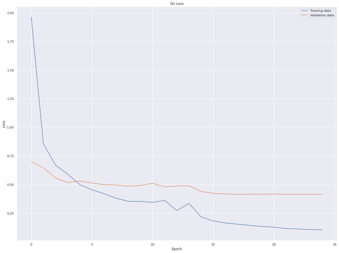
1700/1700 [==============================] - 56s 33ms/step - loss: 0.1048 - accuracy: 0.9579 - val_loss: 0.4161 - val_accuracy: 0.9157 - lr: 4.0000e-0525 epoch에서 학습이 종료되었으며 저장된 값은 22epoch, train_loss는 0.1156, train_accuracy는 0.9562, val_loss는 0.4146, val_accuracy는 0.9153이다. 여전히 train_loss와 val_loss 간의 차이가 크다.
3. 학습 곡선 확인
history에 저장된 내용을 토대로 accuracy와 loss 곡선을 그려보았다.
# 모델 학습 후 정보가 담긴 history 내용을 토대로 선 그래프를 그리는 함수 설정

def plot_acc(history, title=None):        # Accuracy(정확도) Visualization
    # summarize history for accuracy
    if not isinstance(history, dict):
        history = history.history

    plt.plot(history['accuracy'])        # accuracy
    plt.plot(history['val_accuracy'])    # validation accuracy
    if title is not None:
        plt.title(title)
    plt.ylabel('Accracy')
    plt.xlabel('Epoch')
    plt.legend(['Training data', 'Validation data'], loc=0)
    # plt.show()

def plot_loss(history, title=None):     # Loss Visualization
    # summarize history for loss
    if not isinstance(history, dict):
        history = history.history

    plt.plot(history['loss'])           # loss
    plt.plot(history['val_loss'])       # validation
    if title is not None:
        plt.title(title)
    plt.ylabel('Loss')
    plt.xlabel('Epoch')
    plt.legend(['Training data', 'Validation data'], loc=0)
    # plt.show()

plot_acc(history, '(a) Accuracy')  # 학습 경과에 따른 정확도 변화 추이
plt.show()
plot_loss(history, '(b) Loss')     # 학습 경과에 따른 손실값 변화 추이
plt.show()
4. test 셋으로 성능 확인
test 셋을 모델에 넣어 예측하고 F1-score를 통해 모델의 성능을 평가해보았다. macro F1-score는 대회의 평가지표 중 하나로 라벨 별 각 합의 평균을 의미한다. 점수는 0.8588 정도가 나왔다. 이는 대회 1등 지표보다 훨씬 높지만 모델의 한계로 이미 학습과정에서 overfitting이 진행되어 정확한 결과가 아니고 실제로 제출한 점수는 약 0.79정도로 나왔다.
cate_y_test = np.array(pd.get_dummies(test_label).values)

# best_model 불러오기
from tensorflow.keras.models import load_model
model_saved = load_model('/content/drive/MyDrive/StatisticCompetition/oktmorphs/best_model_4.h5')

# 라벨 인덱스 구하기
labels = pd.DataFrame(test_label)
sorted_labels = np.sort(labels[0].unique())  # 정렬된 라벨들 225개
len(sorted_labels)

# test셋에 대한 예측
y_predict = model_saved.predict(test_input)
final_label = []    # 예측한 라벨

for i in range(len(y_predict)):
    index = sorted_labels[y_predict[i].argmax()]
    index2 = y_predict[i][y_predict[i].argmax()]
    final_label.append(index)

from sklearn.metrics import f1_score
print('macro ', f1_score(test_label, final_label, average='macro'))
macro 0.85867101800487545. 결과 제출
# 라벨 인덱스 구하기
labels = pd.DataFrame(train_input)
sorted_labels = np.sort(labels[0].unique())  # 정렬된 라벨들 225개

# submit용 예측하기
submit_predict = model_saved.predict(submit_input)
submit_label = []                                   # 제출용 라벨
for i in range(len(submit_predict)):
    index = sorted_labels[submit_predict[i].argmax()]
    submit_label.append(index)

# 제출 파일 작성
submission_file = pd.read_csv('/content/drive/MyDrive/StatisticCompetition/답안 작성용 파일.csv', encoding = 'cp949')
submission_file['digit_3'] = submit_label
sequences = raw_data[['digit_1', 'digit_2', 'digit_3']]
sequences = sequences.drop_duplicates()                      # 순서쌍 가져오기
final = pd.merge(submission_file, sequences, on='digit_3', how = 'left')
final = final.drop(['digit_1_x', 'digit_2_x'], axis=1)
final.rename(columns={'digit_1_y':'digit_1',
                      'digit_2_y': 'digit_2'}, inplace=True)
final = final[['AI_id', 'digit_1', 'digit_2', 'digit_3', 'text_obj', 'text_mthd', 'text_deal']]
final.to_csv('/content/drive/MyDrive/StatisticCompetition/oktmorphs/submission.csv', encoding='cp949', index=False)
print(final)
AI_id digit_1 digit_2 digit_3 text_obj text_mthd text_deal
0 id_000001 I 56 561 치킨전문점에서 고객의주문에의해 치킨판매
1 id_000002 G 47 475 산업공구 다른 소매업자에게 철물 수공구
2 id_000003 S 94 949 절에서 신도을 대상으로 불교단체운영
3 id_000004 S 96 961 영업장에서 고객요구로 자동차튜닝
4 id_000005 I 56 562 실내포장마차에서 접객시설을 갖추고 소주,맥주제공
... ... ... ... ... ... ... ...
99995 id_099996 A 1 11 사업장에서 일반인대상으로 버섯농장
99996 id_099997 Q 86 862 한의원에서 외래환자위주고 치료
99997 id_099998 G 47 478 일반점포에서 소비자에게 그림판매
99998 id_099999 R 90 902 사업장에서 일반인.학생대상으로 학습공간제공
99999 id_100000 L 68 682 사업장에서 대리현대아파트를 관리
[100000 rows x 7 columns]부족했던 점들..
수업이나 구글링으로 공부하는게 다였다가 제대로 대회에 참여해본 것은 처음이라 많은 어려움들이 있었다. 데이터의 type부터 모델을 돌아가게 만들고 제출 파일을 만드는 과정까지 어느 것 하나 쉬운게 없었다. Pre-trained 에 비해 모델 자체의 한계도 있겠지만 무엇보다 효과적으로 파라미터를 튜닝하고 데이터의 특성에 맞게 모델을 짜는 것에서 다른 참가자들과 일반화 성능에서 차이가 났다고 생각한다.
특히 overfitting을 잡기 위해 많은 제한장치(dropout, regularization, batch normalization, dense layer, initializer)들을 사용하였지만 val 셋에서의 수치와 실제 성능과는 차이가 많이 났다. 이에 대한 요인으로,
-
데이터 셋의 부족 : 100만 개의 많은 데이터셋이 있었지만 클래스 불균형 문제가 심각해 소수 클래스 데이터의 학습을 잘되게 만드는 방법이 부족했다. data resampling 기법인 SMOTE 기법도 고려하였으나 소수 클래스만 upsampling 하는 방법을 찾지 못하였다.
-
과도한 Data Augmentation : 위에선 7만개의 데이터만 augment 하였지만 여러 시행착오 중 120만개의 data를 augment 한 경우 F1-score가 무려 0.92까지 올라가는 기염을 토했다. 싱글벙글하며 하루에 한 번의 기회가 있는 제출점수 확인 결과 오히려 0.73으로 떨어져 그저 overfitting 됐다는 처참한 결론만을 낳았다. 더 많은 데이터를 얻는 것은 좋으나 무분별한 augmentation은 오히려 악영향을 끼친다.
-
Layer 깊이의 부족 : 위에서 1024의 filter 사이즈를 가지는 Convolution layer + MaxPooling layer를 1개만 사용하였다. 하지만 시행착오를 거친 결과 가장 간단한 층이 가장 높은 성능을 보였다. 한글 text 데이터의 CNN 적용 관련 자료가 많지 않아 모델을 구성하는데 한계가 있었고 깊은 층과 일반화 성능을 동시에 가져갈 수 있는 방법이 필요할 것이다.
또한 맨 처음 data를 합치는 과정에서 단순히 3개 컬럼(digit_1(대분류), digit_2(중분류), digit_3(소분류))을 붙이는 것이 맞는 방법인지에 대한 의문도 든다. 하나의 문장으로 생각하고 적용시킨 모델이지만 실제로 문장들을 살펴보면 하나의 한글 문장이라고 생각하기엔 힘들기 때문이다.
결론
비록 대회에서 좋은 결과를 내진 못했지만 많은 것들을 얻을 수 있었다. 기본적으로 데이터를 다루는 방법들, 예를 들면 dataframe의 slicing을 for 문과 적절히 섞어서 원하는 결과물을 뽑는 방법이라던지, text 데이터의 전처리법, CNN의 작동 원리, train과 val셋을 비교하여 학습시키는 법, earlystopping과 같은 overfitting 방지법, 결과물 제출법 등등 아주 많았다. 모델의 선정과 일반화성능을 잡지 못해 점수가 잘 나오지 못한 점은 아쉬웠지만 첫 술에 배부를 순 없는 법, 앞으로도 많은 대회들에 계속해서 도전해 볼 생각이다.
그리고 무엇보다 이런 머신러닝, 딥러닝을 활용하여 모델을 짜고 예측하여 경쟁하는 과정 자체에 큰 흥미를 느끼게 되어 추후의 대회들을 열심히 참여할 원동력이 될 것이라 믿어 의심치 않는다.
References
- Activation Function
- EDA(Easy Data Augmentation)
- CNN 모델
- 클래스 가중치 생성 함수
- (텐서플로2와 머신러닝으로 시작하는) 자연어 처리 : 로지스틱 회귀부터 BERT와 GPT2까지 / 전창욱 / 2020 / 위키북스
- 한국어 임베딩 : 자연어 처리 모델의 성능을 높이는 핵심 비결 Word2Vec에서 ELMo, RT까지 / 이기창 / 2019 / 에이콘출판
