수업 50일차

✔ 군집

문서의 군집 실습

• 데이터
  - https://archive.ics.uci.edu/dataset/191/opinosis+opinion+frasl+review
  

import pandas as pd
import glob ,os
path = './data/OpinosisDataset1.0/topics' 
# path로 지정한 디렉토리 밑에 있는 모든 .data 파일들의 파일명을 리스트로 취합
all_files = glob.glob(os.path.join(path, "*.data")) 
# print(all_files)

# 여기에는 파일의 이름을 모으고
filename_list = []
# 여기에는 내용을 모으자.
opinion_text = []
for file_ in all_files:
    df=pd.read_table(file_,index_col=None, header=0,encoding='latin1')
    # 파일 이름만 추출해보자.
    filename_=file_.split('\\')[-1]
    filename=filename_.split(".")[0]
    # 파일명과 내용을 list에 저장하자
    filename_list.append(filename)
    opinion_text.append(df.to_string())
# print(filename_list[0])
# print(opinion_text[0])
# 파일 이름과 내용으로 DF 생성
document_df=pd.DataFrame({'filename':filename_list,'opinion_text':opinion_text})
document_df.head()

• 피처 벡터화

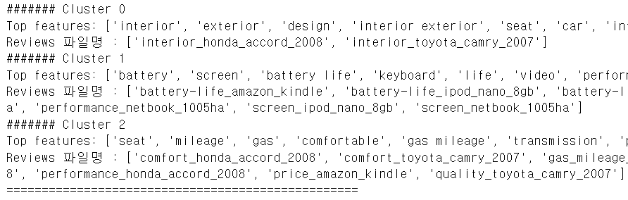
from nltk.stem import WordNetLemmatizer
import nltk
import string
# 구두점 제거
remove_punct_dict=dict((ord(punct),None) for punct in string.punctuation)
# print(remove_punct_dict)
lemmar=WordNetLemmatizer()
def LemTokens(tokens):
    return [lemmar.lemmatize(token) for token in tokens]
def LemNormalize(text):
    return LemTokens(nltk.word_tokenize(text.lower().translate(remove_punct_dict)))

from sklearn.feature_extraction.text import TfidfVectorizer
tfidf_vect = TfidfVectorizer(tokenizer=LemNormalize, stop_words='english' , 
                            ngram_range=(1,2), min_df=0.05, max_df=0.85 )
# 문자에 어떤 단어가 얼마의 가중치를 가지고 있는지 희소 행렬로 생성
feature_vect = tfidf_vect.fit_transform(document_df['opinion_text'])
print(feature_vect)

# 군집 알고리즘 수행
from sklearn.cluster import KMeans
# 5개의 군집을 위한 인스턴스 생성
km_cluster=KMeans(n_clusters=5, max_iter=10000, random_state=0)
# 훈련
km_cluster.fit(feature_vect)
#레이블 저장
cluster_label=km_cluster.labels_
# 중앙점 저장
cluster_centers=km_cluster.cluster_centers_
document_df['cluster_label']=cluster_label
document_df.sort_values(by='cluster_label')
document_df.head()

# 군집을 이루게 만드는 핵심 단어 출력
# 클러스터링 모델과 데이터 그리고 피처 이름, 클러스터 개수 와 
# 추출할 핵심 단어 개수를 받아서 리턴하는 함수
def get_cluster_details(cluster_model, cluster_data, feature_names, clusters_num,
                       top_n_features=10):
    cluster_details={}
    # 군집 중심과의 거리가 먼 단어 순으로 저장하기
    centroid_feature_ordered_ind=cluster_model.cluster_centers_.argsort()[:,::-1]
    for cluster_num in range(clusters_num):
        cluster_details[cluster_num]={}
        cluster_details[cluster_num]['cluster']=cluster_num
        # 실제 중요 피처를 추출
        top_feature_indexes=centroid_feature_ordered_ind[cluster_num,:top_n_features]
        top_features=[feature_names[ind] for ind in top_feature_indexes]
        # 중앙점 과의 거리 저장
        top_feature_values=cluster_model.cluster_centers_[
            cluster_num, top_feature_indexes].tolist()
        cluster_details[cluster_num]['top_features']=top_features
        cluster_details[cluster_num]['top_features_value']=top_feature_values
        filenames=cluster_data[cluster_data['cluster_label']==cluster_num]['filename']
        filenames=filenames.values.tolist()
        cluster_details[cluster_num]['filenames']=filenames
    return cluster_details

# 클러스터 별 핵심 단어를 출력하는 함수
def print_cluster_details(cluster_details):
    for cluster_num, cluster_detail in cluster_details.items():
        print('####### Cluster {0}'.format(cluster_num))
        print('Top features:', cluster_detail['top_features'])
        print('Reviews 파일명 :',cluster_detail['filenames'][:7])
    print('==================================================')

feature_names = tfidf_vect.get_feature_names_out()
cluster_details = get_cluster_details(cluster_model=km_cluster, 
                                      cluster_data=document_df,feature_names=feature_names, 
                                      clusters_num=3, top_n_features=10 )
print_cluster_details(cluster_details)

✔ 문장의 유사도 측정

• 각 문장을 벡터로 만들어서 거리를 측정하는 개념을 이용
  - 코사인 유사도
• 코사인 유사도는 일반적인 거리 측저으이 개념과는 다르고 방향성을 중요시하는 개념
• 두 개의 벡터 간의 사잇각을 구해서 얼마나 유사한지 수치로 적용한 것

sklearn에서 코사인 유사도를 계산하는 방법

• sklearn.feature_extraction.text 패키지를 이용해서 피처 벡터화를 진행하고 sklearn.metrics.pairwise패키지의 cosine_similarity함수를 이용해서 측정합니다.
• 알고리즘 자체는 행렬의 곱셈을 한 뒤, 각 데이터의 제곱값을 더하고 제곱근한 값으로 나누면 됩니다. (그냥 코드를 봐보자)

def cos_similarity(v1,v2):
    dot_product=np.dot(v1,v2)
    l2_norm=(np.sqrt(sum(np.square(v1))))*np.sqrt(sum(np.square(v2)))
    similarity=dot_product/l2_norm
    return similarity

# 거리 계산을 위해서 1차원 배열로 변환
#첫번째 문장과 두번째 문장의 feature vector 추출
vect1 = np.array(feature_vect_dense[0]).reshape(-1,)
vect2 = np.array(feature_vect_dense[1]).reshape(-1,)
vect3 = np.array(feature_vect_dense[2]).reshape(-1,)
#첫번째 문장과 두번째 문장의 feature vector로 두개 문장의 Cosine 유사도 추출
similarity_simple = cos_similarity(vect1, vect2 )
print('문장 1, 문장 2 Cosine 유사도: {0:.3f}'.format(similarity_simple))
similarity_simple = cos_similarity(vect1, vect3 )
print('문장 1, 문장 3 Cosine 유사도: {0:.3f}'.format(similarity_simple))
similarity_simple = cos_similarity(vect2, vect3 )
print('문장 2, 문장 3 Cosine 유사도: {0:.3f}'.format(similarity_simple))

• API 이용 방법도 있다.

# API 를 이용해서 코사인 유사도 계산
from sklearn.metrics.pairwise import cosine_similarity
similarity_simple_pair = cosine_similarity(feature_vect_simple[0] , feature_vect_simple)
print(similarity_simple_pair)

문서 군집의 코사인 유사도 확인

km_cluster=KMeans(n_clusters=3, max_iter=10000, random_state=0)
km_cluster.fit(feature_vect)
cluster_label=km_cluster.labels_
#각 군집의 centroid
cluster_centers=km_cluster.cluster_centers_
document_df['cluster_label_']=cluster_label
print(cluster_centers)

• 각 클러스터마다의 문서들 간 코사인 유사도 확인

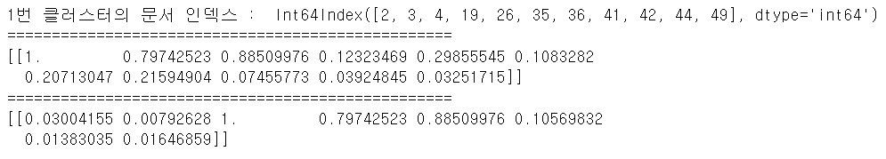
# 1번 클러스터 문서들 간 코사인 유사도 확인
hotel_indexes=document_df[document_df['cluster_label']==1].index
print('1번 클러스터의 문서 인덱스 : ', hotel_indexes)
print('==================================================')
similarity_pair=cosine_similarity(feature_vect[hotel_indexes[0]],
                                 feature_vect[hotel_indexes])
print(similarity_pair)
print('==================================================')
# 0 번 부터 7번까지의 문서와 코사인 유사도
similarity_pair=cosine_similarity(feature_vect[hotel_indexes[0]],
                                 feature_vect[[0,1,2,3,4,5,6,7]])
print(similarity_pair)

한글 문서의 유사도 측정

• 한글은 형태소 분석을 수행해야 합니다.

from sklearn.feature_extraction.text import CountVectorizer
from konlpy.tag import Okt
okt=Okt()
vectorizer=CountVectorizer(min_df=1)
contents=['우리 과일 먹으러 가자', '오늘은 목요일입니다.',
        '나는 한강에서 산책하는 것을 좋아해',
        '나는 강아지랑 놀러가는 것을 좋아해.']
# 한글 토큰화
contents_tokens=[okt.morphs(row) for row in contents]
print(contents_tokens)

# 토큰화 된 결과를 가지고 다시 문장을 생성해야해
# 피처 벡터화 하려면 문장 형태여야 하기 때문이야
contents_for_vectorize=[]
for content in contents_tokens:
    sentence=''
    for word in content:
        sentence=sentence+' '+word
    contents_for_vectorize.append(sentence)
print(contents_for_vectorize)

# 피처 벡터화
X=vectorizer.fit_transform(contents_for_vectorize)
# 피처 확인
print(vectorizer.get_feature_names_out())
# 문장의 피처 벡터화 된 후의 결과 확인
print(X.toarray().transpose())

• 테스트

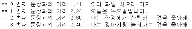
# 테스트 데이터 생성
new_post=['우리 사과 먹으러 가즈아']
new_post_tokens=[okt.morphs(row) for row in new_post]
new_post_for_vectorize=[]
for content in new_post_tokens:
    sentence=''
    for word in content:
        sentence=sentence+' '+word
    new_post_for_vectorize.append(sentence)
print(new_post_for_vectorize)

# 테스트 데이터의 피처 벡터화
new_post_vec=vectorizer.transform(new_post_for_vectorize)
print(new_post_vec)
print(new_post_vec.toarray())

# 거리를 구해주는 함수
import scipy as sp
def dist_raw(v1,v2):
    delta =v1-v2
    return sp.linalg.norm(delta.toarray())

# 다른 문장들 과의 거리 계산
best_doc = None
best_dist = 65535
best_i = None
for i in range(0, 4):
    post_vec = X.getrow(i)
    d = dist_raw(post_vec, new_post_vec)
    print("== %i 번째 문장과의 거리:%.2f : %s" %(i,d,contents[i]))
    if d<best_dist:
        best_dist = d
        best_i = i

✔ 연관 분석

word2vec

CBOW(Continuous Bag of Words)

• 여러 개의 단어를 나열한 뒤, 이 와 관련된 단어를 추정하는 문제
• 문자에서 나오는 n개의 단어 열로부터 다음 단어를 예측하는 것

Skip-Gram

• 특정한 단어로부터 문맥을 구성할 수 있는 단어를 예측하는 방식으로 window size라는 매개변수를 이용해서 단어를 예측

word2vec

• CBOW와 Skip-Gram 방식의 단어 임베딩을 구현한 C++ 라이브러리
• Python 에서는 gensim 패키지의 Word2Vec이라는 클래스를 이용해서 제공
• 문장들을 매개변수로 받아서 유사도 계산을 해주고, 가장 유사한 문장을 리턴해주는 기능을 제공하며, positive와 negative 인수를 사용해서 관계도 찾을 수 있다.

네이버 지식인 데이터를 크롤링해서 단어 추천하기

• https://search.naver.com/search.naver?where=kin&sm=tab_jum&ie=utf8&query=검색어&start=인덱스

from bs4 import BeautifulSoup
import urllib
import requests
import time
headers = {'User-Agent': 'Mozilla/5.0 (Windows NT 10.0; Win64; x64) AppleWebKit/537.36 (KHTML, like Gecko) Chrome/116.0.0.0 Safari/537.36'}
# 크롤링 할 문자열을 저장할 list
textlist = []
# 크롤링 할 url 생성
start = 1
query = '윤하노래 추천'
target_url=f"https://search.naver.com/search.naver?where=kin&kin_display=10&query={urllib.parse.quote(query)}&start={start}"
#main_pack > section > div > ul > li:nth-child(1) > div > div.question_area > div.question_group > a
#main_pack > section > div > ul > li:nth-child(1) > div > div.answer_area > div.answer_group > a
# 10개씩 1000개의 url 읽기
for n in range(1, 4):
    start = 1 + (n - 1) * 10
    print("페이지", n)
#     target_url = "https://search.naver.com/search.naver?where=kin&kin_display=10&qt=&title=0&&answer=0&grade=0&choice=0&sec=0&nso=so%3A-1%2Ca%3A%2Cp%3Aall&query=" + urllib.parse.quote('LG채용') + "&c_name=&sm=tab_pge&kin_start=" + str(data) + "&kin_age="
    target_url=f"https://search.naver.com/search.naver?where=kin&kin_display=10&query={urllib.parse.quote(query)}&start={start}"
    response = requests.get(target_url, headers=headers)
    # 파싱
    soup = BeautifulSoup(response.text, 'html.parser')
    for i in range(1, 11):
        print(f"{i}번 글")
        tmp = soup.select('li:nth-child('+str(i)+') > div > div.answer_area > div.answer_group > a')
        if tmp:
            for line in tmp:
                print(line.text)
                textlist.append(line.text)
        else:
            print("엘리먼트를 찾을 수 없습니다.")

• 형태소 분석

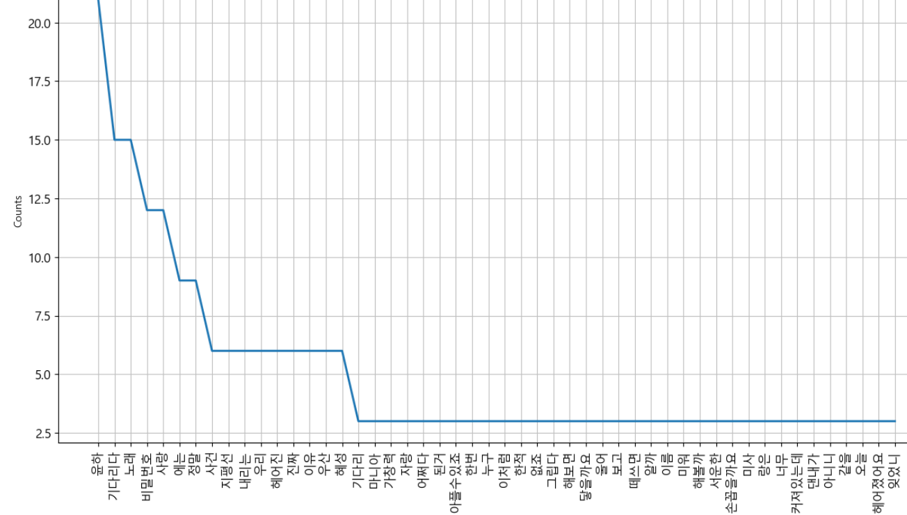
# 형태소 분석
from konlpy.tag import Okt
import re
# 정규식을 사용하여 한글만 추출하는 함수
def extract_korean(text):
    hangul_pattern = re.compile('[가-힣]+')
    return "".join(hangul_pattern.findall(text))
okt=Okt()
# 한글 형태소 분석기는 하나의 문장에만 가능하기에 
# list 데이터를 한 문장으로 변경
present_text=''
for line in textlist:
    hangul_text = extract_korean(line)
    present_text=present_text+hangul_text+'\n'
tokens_ko=okt.morphs(present_text)
print(tokens_ko)

# 형태소 분석 결과를 가지고 등장 횟수 확인
import nltk
ko=nltk.Text(tokens_ko,name="윤하")
print(ko.vocab().most_common(100))

#stopwords
stop_words=['\n', '추천','작곡','다비','드립니다','드릴께요','있을','정도','합니다','이렇게','어떻게','세곡','안녕하세요','김동률','고천']
tokens_ko = [each_word for each_word in tokens_ko if each_word not in stop_words and len(each_word) > 1]
print(tokens_ko)
ko=nltk.Text(tokens_ko,name="윤하")
print(ko.vocab().most_common(100))

plt.figure(figsize=(15,8))
ko.plot(50)
plt.show()

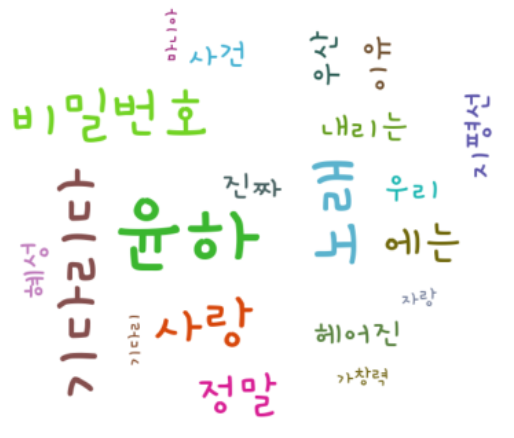
• tagcloud 생성

import pytagcloud
#자주 등장하는 단어 추출
data = ko.vocab().most_common(20)
taglist = pytagcloud.make_tags(data, maxsize=100)
#태그 클라우드 생성
pytagcloud.create_tag_image(taglist, 'wordcloud_YH.png', size=(700, 600),
                            fontname="Korean_Gamja", rectangular=False)
import matplotlib.pyplot
import matplotlib.image
img = matplotlib.image.imread('wordcloud_YH.png')
imgplot = matplotlib.pyplot.imshow(img)
plt.axis('off')
matplotlib.pyplot.show()

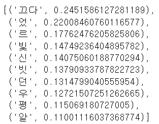
• gensim

# 연관 단어 추출
# 단어의 연관성을 가진 패키지
!pip install gensim

from gensim.models import word2vec
lines=present_text
okt=Okt()
results=[]
for line in lines:
    # 품사 분석을 해서 조사 어미 punctuation(구두점)제거
    malist=okt.pos(line,norm=True, stem=True)
    r=[]
    for word in malist:
        if not word[1] in ["Josa","Eomi","Punctuation"]:
            r.append(word[0])
    r1=(" ".join(r)).strip()
    results.append(r1)
    #print(r1)

data_file='YH.data'
with open(data_file, 'w', encoding='utf-8') as fp:
    fp.write("\n".join(results))
    data = word2vec.LineSentence(data_file)
model=word2vec.Word2Vec(data, vector_size=200, window=10, hs=1, min_count=2, sg=1)
# 모델 저장
model.save("YH.model")
model=word2vec.Word2Vec.load("YH.model")

# 모델의 어휘 확인 (Gensim 4.0.0 이상)
vocabulary = model.wv.key_to_index
# 어휘에 포함된 단어 목록 출력
word_list = list(vocabulary.keys())
print(word_list)

# 연관된 단어 추출 - "밉다" 와 연관 관계가 긍정적으로 높은 10개 단어 추출
model.wv.most_similar(positive=['밉다'])

연관 규칙 분석

• 원본 데이터에서 대상들의 연관된 규칙을 찾는 무방향성 데이터 마이닝 기법
• 하나의 거래나 사건에 포함된 항목 간의 관련성을 찾아서 둘 이상의 항목들로 구성된 연관성 규칙을 도축하는 탐색적 기법
• 트랜잭션을 대상으로 트랜잭션 내의 연관성을 분석해서 거래의 규칙이나 패턴을 찾아내는 분석 방법

장점

• 조건 반응 표현식의 결과를 이해하기 쉬움
• 비목적성 분석이 용이하다

단점

• 계산 시간이 오래 걸림
• 적절한 품목의 결정이 어려움
  - 거래량이 적은 품목과 많은 품목에 대한 상대성 차이에 의한 결과가 다르게 나타날 수 있고, 규칙을 발견하기 어려움
  

활용분야

• 고객 대상 상품 추천 및 상품 정보 발송
• 염기 서열 분석 과 질병의 관계
• 의료비 허위 청구 순서 패턴 분석
• 불량 유발 공정 및 장비 패턴 탐지
• 웹 사이트의 메뉴 별 클릭 순서

분석절차

• 거래내역 데이터를 대상으로 트랜잭션 객체 생성
• 품목과 트랜잭션ID 확인
• 지지도, 신뢰도, 향상도를 이용한 연관 규칙 발견
• 연관 규칙에 대한 시각화 - 네트워크 시각화
• 연관 분석 결과를 해설 및 업무 적용

연관 규칙 평가 척도

• Support (지지도)
  - n(X^Y)/N
  - 전체 거래 개수에서 X와 Y가 모두 포함된 건수의 비율
  - 전체 품목에서 X와 Y가 모두 구매한 거래확률
  - 지지도가 낮다는 것은 거래가 자주 발생하지 않는다는 의미
  - X Y 순서를 변경해도 값은 그대로
• Confidence (신뢰도)
  - n(X^Y)/n(X)
  - X를 구매한 거래 중 Y도 구매한 경우
  - 지지도는 포함 비중이 낮으면 연관성을 파악하기가 어려움
• Lift(향상도)
  - c(X->Y)/s(Y)
  - 두 항목의 독립성 여부를 수치로 제공
  - 이 값이 1이면 완전 독립
  - 이 값이 1보다 작으면 음의 상관 관계
  - 이 값이 1보다 크면 양의 상관 관계로 같이 구매할 확률이 높아지는 것
• 파이썬에서는 apyori 패키지를 이용해서 제공
  - 하나의 트랜잭션을 list를 만들고 이 들의 list를 가지고 rule을 생성
  - 인스턴스를 만들 때 지지도, 향상도, 신뢰도를 설정할 수 있습니다.

tweet_temp.csv 파일 내용을 가지고 연관 규칙 분석 수행하기

• 데이터 로드

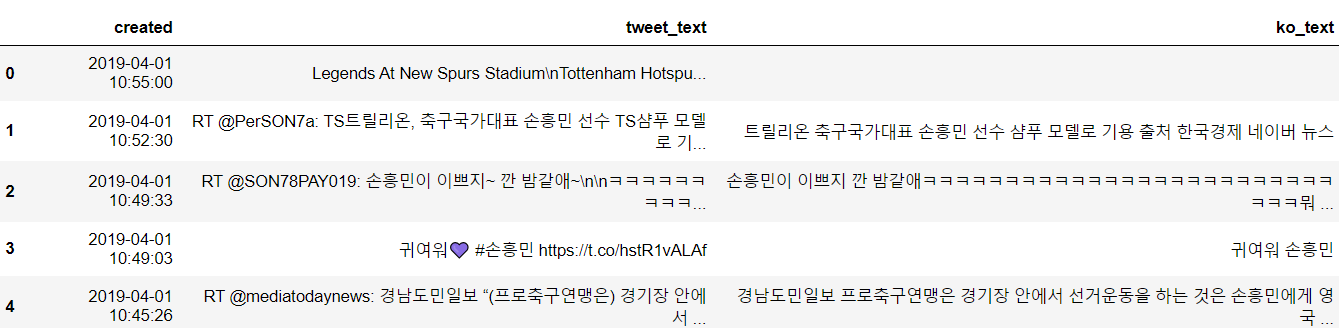
df=pd.read_csv('./data/tweet_temp.csv')
df.head()
# 시간과 실제 트윗 내용이다.

• 데이터 전처리

# 한글만 추출하기
import re
def text_cleaning(text):
    # 한글 정규표현식
    hangul=re.compile('[^ㄱ-ㅣ 가-힣]+')
    # 한글 아닌 것은 전부 ''로 치환하기
    result=hangul.sub('',text)
    return result
df['ko_text']=df['tweet_text'].apply(lambda x : text_cleaning(x))
df.head()

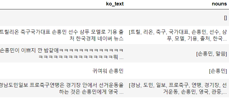
# 한글을 쓴다면 이제 형태소 분석은 무조건이다.
from konlpy.tag import Okt
from collections import Counter
# 한국어 불용어사전 만들기
# https://www.ranks.nl/stopwords/korean
# 메모장에 해서 해도 됨
korean_stopwords_path='./data/stopwords.txt'
with open(korean_stopwords_path, encoding='utf-8') as f:
    stopwords=f.readlines()
stopwords=[x.strip() for x in stopwords]
# print(stopwords)

def get_nouns(x):
    # 형태소 분석
    nouns_tagger=Okt()
    nouns=nouns_tagger.nouns(x)
    # 한 글자 제거
    nouns=[noun for noun in nouns if len(noun)>1]
    # 불용어 제거
    nouns = [noun for noun in nouns if noun not in stopwords]
    return nouns
df['nouns']=df['ko_text'].apply(lambda x : get_nouns(x))
df.head()

# 연관 분석 수행
!pip install apyori

• 별다른 옵션 없이 연관 규칙 분석 수행하기

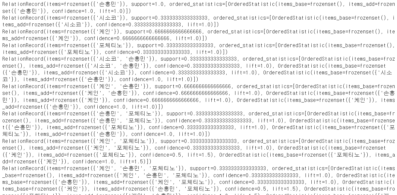
# 거래 생성
transactions=[['손흥민','케인'],['손흥민','시소코'],
             ['손흥민','포체티노','케인']]
from apyori import apriori
results=list(apriori(transactions))
for result in results:
    print(result)

• 옵션을 걸어보자.

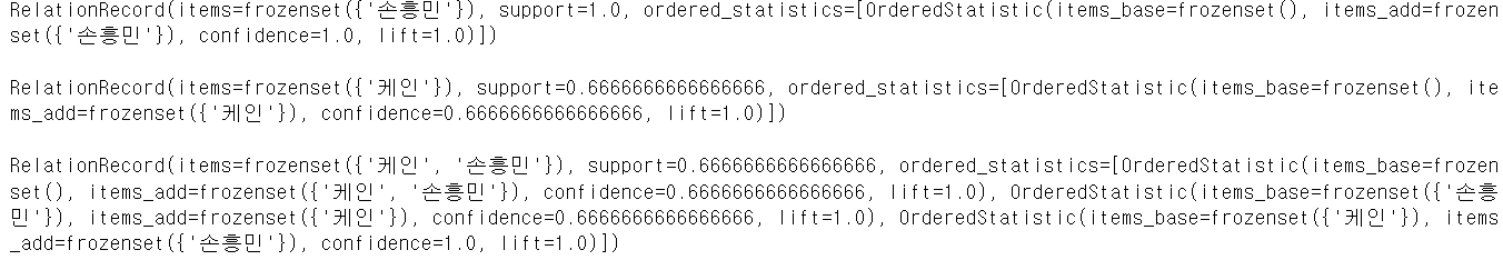
# 이번엔 옵션을 걸어보자
# 지지도 0.5 이상, 향상도 1.0 이상, 신뢰도 0.6 이상인 거래만 확인
results=list(apriori(transactions,min_support=0.5,
                    min_confidence=0.6,
                    min_lift=1.0, max_length=2))
for result in results:
    print(result)
    print()

• 확 줄어버린다.

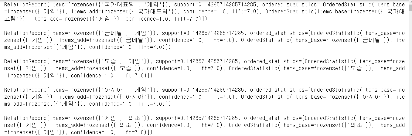
# 데이터프레임의 데이터를 list로 변환
transactions=df['nouns'].tolist()
transactions=[transaction for transaction in transactions if transaction]
results=list(apriori(transactions, min_support=0.1, 
                    min_confidence=0.2, min_lift=5,
                    max_length=2))
for result in results:
    print(result)
    print()

• 한개의 상품만 있는 것도 있다.
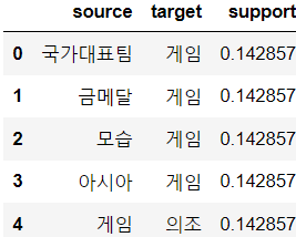
• 보기 조금 어렵다.

# 결과를 데이터프레임으로 변환하고 
# 한개의 상품만 있는 경우는 제거하자(의미 X)
columns=['source', 'target', 'support']
network_df=pd.DataFrame(columns=columns)
for result in results:
    if len(result.items)==2:
        # 결과의 item 이름을 가지고 와서 리스트로 생성
        items=[x for x in result.items]
        row=[items[0], items[1], result.support]
        # 시리즈로 변환
        series=pd.Series(row, index=network_df.columns)
        network_df=network_df.append(series, ignore_index=True)
network_df.head()

네트워크 시각화를 해보자.

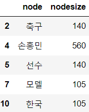
tweet_corpus=''.join(df['ko_text'].tolist())
print(tweet_corpus)

nouns_tagger=Okt()
nouns=nouns_tagger.nouns(tweet_corpus)
count=Counter(nouns)
remove_char_counter=Counter({x:count[x] for x in count if len(x)>1})
print(remove_char_counter)

# 데이터가 많으니까 노드사이즈 50이상 애들만 가져가자
node_df=pd.DataFrame(remove_char_counter.items(), columns=['node', 'nodesize'])
node_df=node_df[node_df['nodesize']>=50]
node_df.head()

• 단어가 노드, 등장횟수가 노드 사이즈가 된다.

# 네트워크 시각화 패키지를 설치하자
!pip install networkx

1

✔ 추천 시스템

구현 방법

• Contents Based Filtering(컨텐츠 기반)
  - 사용자가 특정한 아이템을 선호하는 경우, 그 아이템과 유사한 콘텐츠를 가진 다른 아이템을 추천하는 방식
• Collaborative Filtering(협업 필터링)
  - 사용자가 아이템에 매긴 평점 정보나 구매 이력 등을 기반으로 사용자 행동 양식만을 기반으로 만드는 방식
  - 사용자와 아이템 평점 매트릭스가 있다면, 사용자가 특정 아이템에 매긴 평점을 가지고 아직 사용자가 매기지 않은 아이템에 대해서 평점을 예측하는 방식
  - 이 방식은 주로 희소행렬을 이용합니다.
  - Nearest Neighbor(최근접 이웃) 협업 필터링
  - Latent Factor(잠재 요인) 협업 필터링

  ---

• 예전에는 콘텐츠 기반 필터링과 최근접 이웃이 많이 사용되었는데, 넷플릭스 추천 대회에서 행렬 분해를 이용한 Latent Factor가 우승하면서 최근에 많이 사용하고 있다.
• 최근에는 여기서도 앙상블 기법처럼 콘텐츠 기반 필터링과 협업 기반 필터링을 같이 사용하기도 합니다.

잠재요인 협업 필터링

• 사용자를 행으로 놓고 각 아이템을 열(피처)에 배치
• 사용자는 거의 모든 피처에 None을 소유
• 주성분 분석과 같은 차원 축소를 해서 None이 거의 없을 것이고 이를 복원하게 된다면 빈자리에 값이 채워지게 됩니다.
• 차원 축소를 할 때 행렬분해 사용

콘텐츠 기반 필터링

• 데이터 : https://www.kaggle.com/datasets/tmdb/tmdb-movie-metadata