
✔ 추천 시스템
상품 추천
# 영국 선물샵 온라인 도매 거래 데이터
df = pd.read_csv("./data/online_retail.csv", dtype={'CustomerID': str,'InvoiceID': str}, encoding="ISO-8859-1")
#데이터의 자료형 변환
df['InvoiceDate'] = pd.to_datetime(df['InvoiceDate'], format="%m/%d/%Y %H:%M")
df.head()
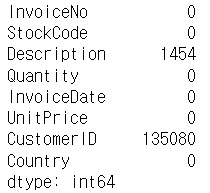
df.info()
df.isnull().sum()
- 데이터 전처리
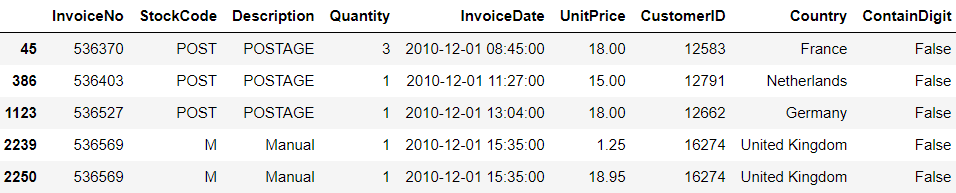
#결측치 제거
df = df.dropna()
print(df.shape)
#상품 수량이 음수인 경우를 제거
print(df[df['Quantity']<=0].shape[0])
df = df[df['Quantity']>0]
#상품 가격이 0 이하인 경우를 제거
print(df[df['UnitPrice']<=0].shape[0])
df = df[df['UnitPrice']>0]
# 상품 코드가 일반적이지 않은 경우를 탐색
df['ContainDigit'] = df['StockCode'].apply(lambda x: any(c.isdigit() for c in x))
print(df[df['ContainDigit'] == False].shape[0])
df[df['ContainDigit'] == False].head()
# 상품 코드가 일반적이지 않은 경우를 제거합니다.
df = df[df['ContainDigit'] == True]
- 탐색적 데이터 분석
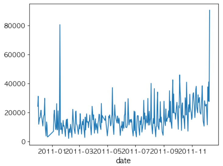
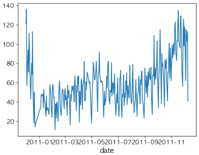
# 거래 데이터에서 가장 오래된 데이터와 가장 최신의 데이터를 탐색
df['date'] = df['InvoiceDate'].dt.date
print(df['date'].min())
print(df['date'].max())
# 일자별 총 거래 수량을 탐색
date_quantity_series = df.groupby('date')['Quantity'].sum()
date_quantity_series.plot()
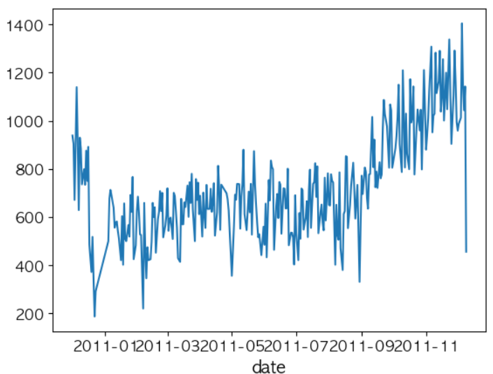
# 일자별 총 거래 횟수를 탐색
date_transaction_series = df.groupby('date')['InvoiceNo'].nunique()
date_transaction_series.plot()
# 일자별 거래된 상품의 unique한 갯수, 즉 상품 거래 다양성을 탐색
date_unique_item_series = df.groupby('date')['StockCode'].nunique()
date_unique_item_series.plot()
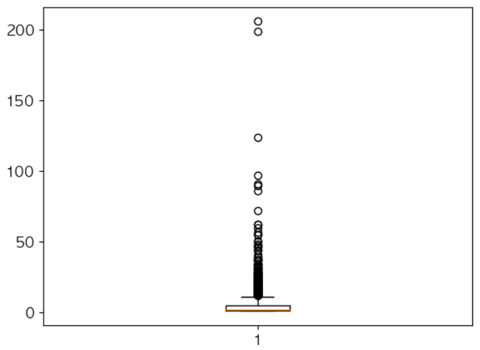
# 총 유저의 수를 계산하여 출력
print(len(df['CustomerID'].unique()))
# 유저별 거래 횟수를 탐색
customer_unique_transaction_series = df.groupby('CustomerID')['InvoiceNo'].nunique()
customer_unique_transaction_series.describe()
# 상자 그림 시각화
plt.boxplot(customer_unique_transaction_series.values)
plt.show()
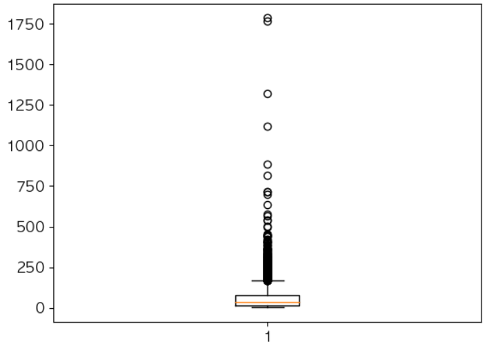
#  유저별 아이템 구매 종류 개수를 탐색
customer_unique_item_series = df.groupby('CustomerID')['StockCode'].nunique()
customer_unique_item_series.describe()
# 상자 그림 시각화
plt.boxplot(customer_unique_item_series.values)
plt.show()
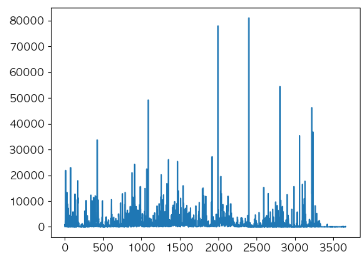
# 총 상품 갯수를 탐색
print(len(df['StockCode'].unique()))
# 가장 거래가 많은 상품 top 10 탐색
df.groupby('StockCode')['InvoiceNo'].nunique().sort_values(ascending=False)[:10]
# 상품별 판매수량 분포를 탐색
print(df.groupby('StockCode')['Quantity'].sum().describe())
plt.plot(df.groupby('StockCode')['Quantity'].sum().values)
plt.show()
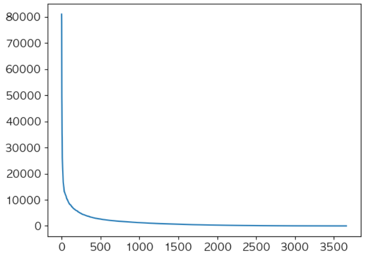
# 분포를 정렬하여 출력
plt.plot(df.groupby('StockCode')['Quantity'].sum().sort_values(ascending=False).values)
plt.show()
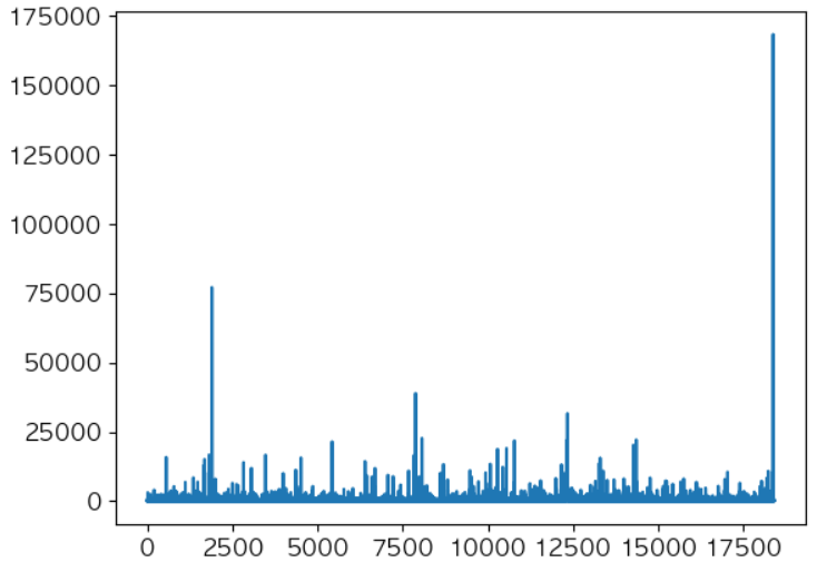
# 거래별로 발생한 가격에 대해 탐색
df['amount'] = df['Quantity'] * df['UnitPrice']
df.groupby('InvoiceNo')['amount'].sum().describe()
# 거래별로 발생한 가격 분포를 탐색
plt.plot(df.groupby('InvoiceNo')['amount'].sum().values)
plt.show()
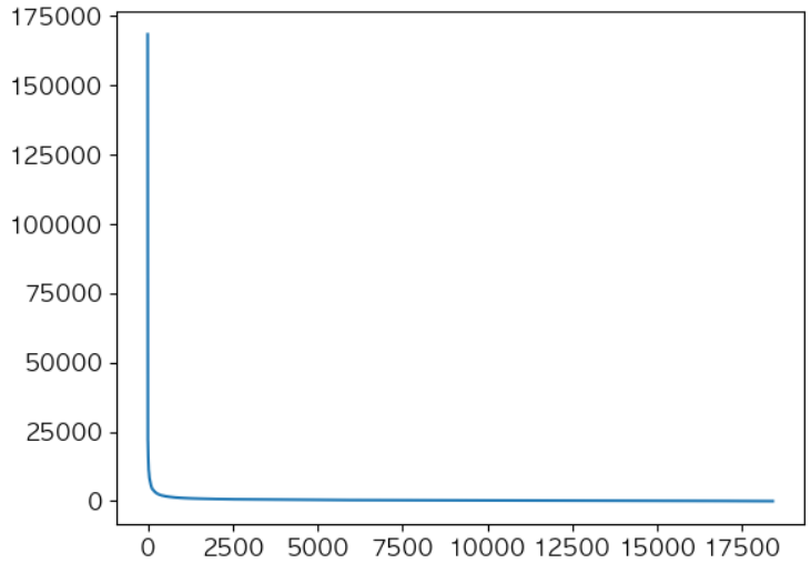
# 분포를 정렬하여 출력
plt.plot(df.groupby('InvoiceNo')['amount'].sum().sort_values(ascending=False).values)
plt.show()
import datetime
# 2011년 11월을 기준으로 하여, 기준 이전과 이후로 데이터를 분리
df_year_round = df[df['date'] < datetime.date(2011, 11, 1)]
df_year_end = df[df['date'] >= datetime.date(2011, 11, 1)]
print(df_year_round.shape)
print(df_year_end.shape)
# 11월 이전 데이터에서 구매했던 상품의 set을 추출 customer_item_round_set = df_year_round.groupby('CustomerID')['StockCode'].apply(set) print(customer_item_round_set)# 11월 이전에 구매했는지 혹은 이후에 구매했는지를 유저별로 기록하기 위한 사전을 정의 customer_item_dict = {} # 11월 이전에 구매한 상품은 'old'라고 표기합니다. for customer_id, stocks in customer_item_round_set.items(): customer_item_dict[customer_id] = {} for stock_code in stocks: customer_item_dict[customer_id][stock_code] = 'old' print(str(customer_item_dict)[:100] + "...")# 11월 이후 데이터에서 구매하는 상품의 set을 추출 customer_item_end_set = df_year_end.groupby('CustomerID')['StockCode'].apply(set) print(customer_item_end_set)# 11월 이전에만 구매한 상품은 'old', 이후에만 구매한 상품은 'new', 모두 구매한 상품은 'both'라고 표기 for customer_id, stocks in customer_item_end_set.items(): # 11월 이전 구매기록이 있는 유저인지를 체크 if customer_id in customer_item_dict: for stock_code in stocks: # 구매한 적 있는 상품인지를 체크한 뒤, 상태를 표기 if stock_code in customer_item_dict[customer_id]: customer_item_dict[customer_id][stock_code] = 'both' else: customer_item_dict[customer_id][stock_code] = 'new' # 11월 이전 구매기록이 없는 유저라면 모두 'new'로 표기 else: customer_item_dict[customer_id] = {} for stock_code in stocks: customer_item_dict[customer_id][stock_code] = 'new' print(str(customer_item_dict)[:100] + "...")# 'old', 'new', 'both'를 유저별로 탐색하여 데이터 프레임을 생성 columns = ['CustomerID', 'old', 'new', 'both'] df_order_info = pd.DataFrame(columns=columns) # 데이터 프레임을 생성하는 과정 for customer_id in customer_item_dict: old = 0 new = 0 both = 0 # 딕셔너리의 상품 상태(old, new, both)를 체크하여 데이터 프레임에 append 할 수 있는 형태로 처리 for stock_code in customer_item_dict[customer_id]: status = customer_item_dict[customer_id][stock_code] if status == 'old': old += 1 elif status == 'new': new += 1 else: both += 1 # df_order_info에 데이터를 append row = [customer_id, old, new, both] series = pd.Series(row, index=columns) df_order_info = df_order_info.append(series, ignore_index=True) df_order_info.head()# 데이터 프레임에서 전체 유저 수를 출력 print(df_order_info.shape[0]) # 데이터 프레임에서 old가 1 이상이면서, new가 1 이상인 유저 수를 출력 # 11월 이후에 기존에 구매한적 없는 새로운 상품을 구매한 유저를 의미 print(df_order_info[(df_order_info['old'] > 0) & (df_order_info['new'] > 0)].shape[0]) # 데이터 프레임에서 both가 1 이상인 유저 수를 출력 # 재구매한 상품이 있는 유저 수를 의미 print(df_order_info[df_order_info['both'] > 0].shape[0])# new 피처의 value_counts를 출력하여, 새로운 상품을 얼마나 구매하는지 탐색 df_order_info['new'].value_counts() # 만약 새로운 상품을 구매한다면, 얼마나 많은 종류의 새로운 상품을 구매하는지 탐색 print(df_order_info['new'].value_counts()[1:].describe())
- SVD를 이용한 상품 구매 예측
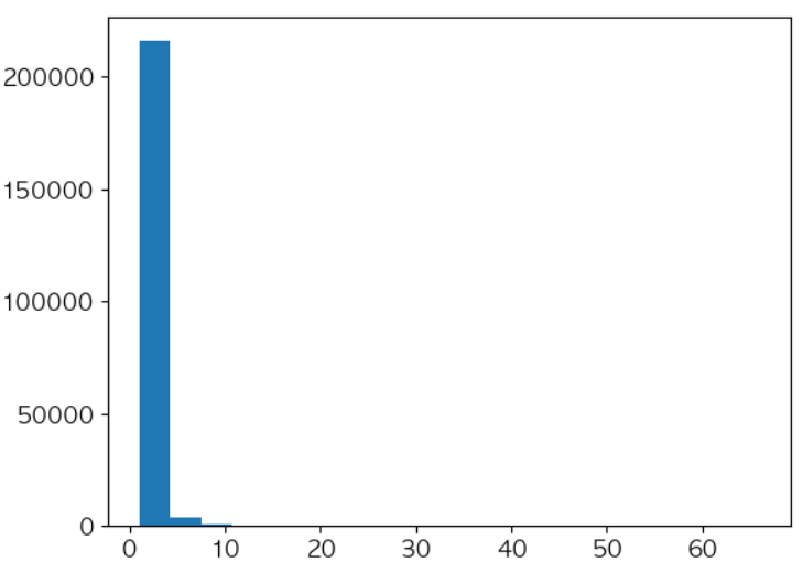
# 추천 대상 데이터에 포함되는 유저와 상품의 갯수를 출력
print(len(df_year_round['CustomerID'].unique()))
print(len(df_year_round['StockCode'].unique()))
# Rating 데이터를 생성하기 위한 탐색 : 유저-상품간 구매 횟수를 탐색
uir_df = df_year_round.groupby(['CustomerID', 'StockCode'])['InvoiceNo'].nunique().reset_index()
uir_df.head()
# Rating(InvoiceNo) 피처의 분포를 탐색 uir_df['InvoiceNo'].hist(bins=20, grid=False)
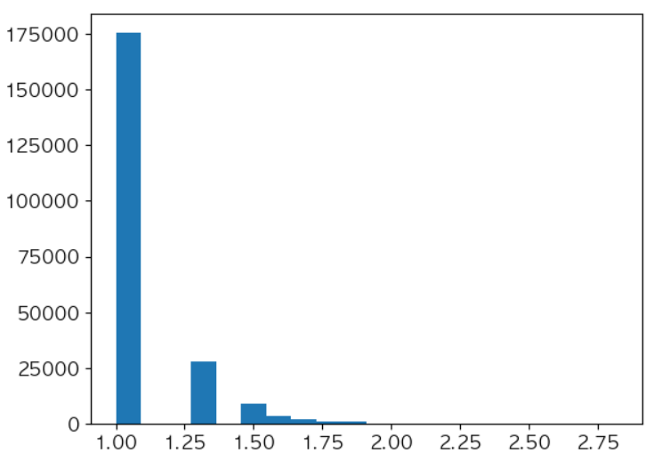
# Rating(InvoiceNo) 피처를 log normalization 해준 뒤, 다시 분포를 탐색
uir_df['InvoiceNo'].apply(lambda x: np.log10(x)+1).hist(bins=20, grid=False)
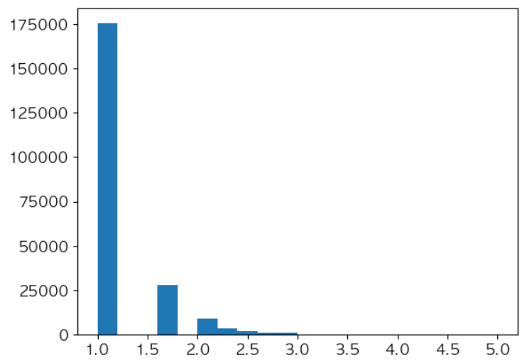
# 1~5 사이의 점수로 변환
uir_df['Rating'] = uir_df['InvoiceNo'].apply(lambda x: np.log10(x)+1)
uir_df['Rating'] = ((uir_df['Rating'] - uir_df['Rating'].min()) /
                    (uir_df['Rating'].max() - uir_df['Rating'].min()) * 4) + 1
uir_df['Rating'].hist(bins=20, grid=False)
# SVD 모델 학습을 위한 데이터셋을 생성
uir_df = uir_df[['CustomerID', 'StockCode', 'Rating']]
uir_df.head()
import time from surprise import SVD, Dataset, Reader, accuracy from surprise.model_selection import train_test_split # SVD 라이브러리를 사용하기 위한 학습 데이터를 생성 # 대략적인 성능을 알아보기 위해 학습 데이터와 테스트 데이터를 8:2로 분할 reader = Reader(rating_scale=(1, 5)) data = Dataset.load_from_df(uir_df[['CustomerID', 'StockCode', 'Rating']], reader) train_data, test_data = train_test_split(data, test_size=0.2) # SVD 모델을 학습 train_start = time.time() model = SVD(n_factors=8, lr_all=0.005, reg_all=0.02, n_epochs=200) model.fit(train_data) train_end = time.time() print("training time of model: %.2f seconds" % (train_end - train_start)) predictions = model.test(test_data) # 테스트 데이터의 RMSE를 출력하여 모델의 성능을 평가 print("RMSE of test dataset in SVD model:") accuracy.rmse(predictions)# SVD 라이브러리를 사용하기 위한 학습 데이터를 생성 #11월 이전 전체를 full trainset으로 활용 reader = Reader(rating_scale=(1, 5)) data = Dataset.load_from_df(uir_df[['CustomerID', 'StockCode', 'Rating']], reader) train_data = data.build_full_trainset() # SVD 모델을 학습합니다. train_start = time.time() model = SVD(n_factors=8, lr_all=0.005, reg_all=0.02, n_epochs=200) model.fit(train_data) train_end = time.time() print("training time of model: %.2f seconds" % (train_end - train_start))
상품 추천 시뮬레이션
"""
11월 이전 데이터에서 유저-상품에 대한 Rating을 기반으로 추천 상품을 선정
1. 이전에 구매하지 않았던 상품 추천 : anti_build_testset()을 사용
2. 이전에 구매했던 상품 다시 추천 : build_testset()을 사용
3. 모든 상품을 대상으로 하여 상품 추천
"""
# 이전에 구매하지 않았던 상품을 예측의 대상으로 선정
test_data = train_data.build_anti_testset()
target_user_predictions = model.test(test_data)
# 구매 예측 결과를 딕셔너리 형태로 변환
new_order_prediction_dict = {}
for customer_id, stock_code, _, predicted_rating, _ in target_user_predictions:
    if customer_id in new_order_prediction_dict:
        if stock_code in new_order_prediction_dict[customer_id]:
            pass
        else:
            new_order_prediction_dict[customer_id][stock_code] = predicted_rating
    else:
        new_order_prediction_dict[customer_id] = {}
        new_order_prediction_dict[customer_id][stock_code] = predicted_rating
print(str(new_order_prediction_dict)[:300] + "...")
- 이전에 구매했던 제품과 이전에 구매하지 않았던 제품을 분할할 수 있습니다.
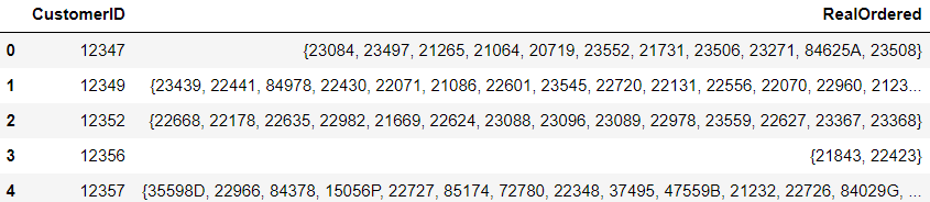
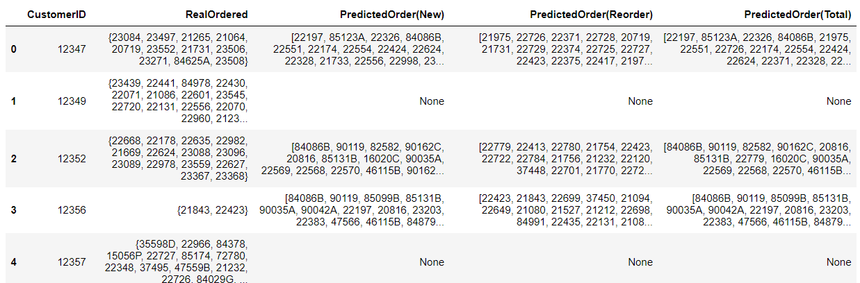
# 이전에 구매했었던 상품을 예측의 대상으로 선정
test_data = train_data.build_testset()
target_user_predictions = model.test(test_data)
# 구매 예측 결과를 딕셔너리 형태로 변환
reorder_prediction_dict = {}
for customer_id, stock_code, _, predicted_rating, _ in target_user_predictions:
    if customer_id in reorder_prediction_dict:
        if stock_code in reorder_prediction_dict[customer_id]:
            pass
        else:
            reorder_prediction_dict[customer_id][stock_code] = predicted_rating
    else:
        reorder_prediction_dict[customer_id] = {}
        reorder_prediction_dict[customer_id][stock_code] = predicted_rating
print(str(reorder_prediction_dict)[:300] + "...")
# 두 딕셔너리를 하나로 통합 total_prediction_dict = {} # new_order_prediction_dict 정보를 새로운 딕셔너리에 저장 for customer_id in new_order_prediction_dict: if customer_id not in total_prediction_dict: total_prediction_dict[customer_id] = {} for stock_code, predicted_rating in new_order_prediction_dict[customer_id].items(): if stock_code not in total_prediction_dict[customer_id]: total_prediction_dict[customer_id][stock_code] = predicted_rating # reorder_prediction_dict 정보를 새로운 딕셔너리에 저장 for customer_id in reorder_prediction_dict: if customer_id not in total_prediction_dict: total_prediction_dict[customer_id] = {} for stock_code, predicted_rating in reorder_prediction_dict[customer_id].items(): if stock_code not in total_prediction_dict[customer_id]: total_prediction_dict[customer_id][stock_code] = predicted_rating print(str(total_prediction_dict)[:300] + "...")# 11월 이후의 데이터를 테스트 데이터셋으로 사용하기 위한 데이터프레임을 생성 simulation_test_df = df_year_end.groupby('CustomerID')['StockCode'].apply(set).reset_index() simulation_test_df.columns = ['CustomerID', 'RealOrdered'] simulation_test_df.head()
# 이 데이터프레임에 상품 추천 시뮬레이션 결과를 추가하기 위한 함수를 정의
def add_predicted_stock_set(customer_id, prediction_dict):
    if customer_id in prediction_dict:
        predicted_stock_dict = prediction_dict[customer_id]
        # 예측된 상품의 Rating이 높은 순으로 정렬
        sorted_stocks = sorted(predicted_stock_dict, key=lambda x : predicted_stock_dict[x], reverse=True)
        return sorted_stocks
    else:
        return None
# 상품 추천 시뮬레이션 결과를 추가
simulation_test_df['PredictedOrder(New)'] = simulation_test_df['CustomerID']. \
                                            apply(lambda x: add_predicted_stock_set(x, new_order_prediction_dict))
simulation_test_df['PredictedOrder(Reorder)'] = simulation_test_df['CustomerID']. \
                                            apply(lambda x: add_predicted_stock_set(x, reorder_prediction_dict))
simulation_test_df['PredictedOrder(Total)'] = simulation_test_df['CustomerID']. \
                                            apply(lambda x: add_predicted_stock_set(x, total_prediction_dict))
simulation_test_df.head()
- 모델 평가하기
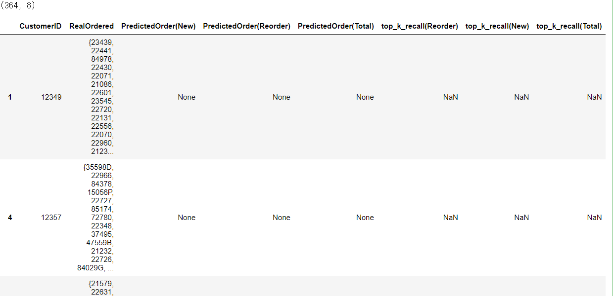
# 구매 예측의 상위 k개의 recall(재현율)을 평가 기준으로 정의합니다.
def calculate_recall(real_order, predicted_order, k):
    # 만약 추천 대상 상품이 없다면, 11월 이후에 상품을 처음 구매하는 유저입니다.
    if predicted_order is None:
        return None
    # SVD 모델에서 현재 유저의 Rating이 높은 상위 k개의 상품을 "구매 할 것으로 예측"합니다.
    predicted = predicted_order[:k]
    true_positive = 0
    for stock_code in predicted:
        if stock_code in real_order:
            true_positive += 1
    # 예측한 상품 중, 실제로 유저가 구매한 상품의 비율(recall)을 계산합니다.
    recall = true_positive / len(predicted)
    return recall
# 시뮬레이션 대상 유저에게 상품을 추천해준 결과를 평가합니다.
simulation_test_df['top_k_recall(Reorder)'] = simulation_test_df. \
                                                apply(lambda x: calculate_recall(x['RealOrdered'],
                                                                                 x['PredictedOrder(Reorder)'],
                                                                                 5), axis=1)
simulation_test_df['top_k_recall(New)'] = simulation_test_df. \
                                                apply(lambda x: calculate_recall(x['RealOrdered'],                                                                          x['PredictedOrder(New)'],
                                                                                 5), axis=1)
simulation_test_df['top_k_recall(Total)'] = simulation_test_df. \
                                                apply(lambda x: calculate_recall(x['RealOrdered'],
                                                                                 x['PredictedOrder(Total)'],                                                                    5), axis=1)
# 평가 결과를 유저 평균으로 살펴보기 print(simulation_test_df['top_k_recall(Reorder)'].mean()) print(simulation_test_df['top_k_recall(New)'].mean()) print(simulation_test_df['top_k_recall(Total)'].mean())# 평가 결과를 점수 기준으로 살펴보기 simulation_test_df['top_k_recall(Reorder)'].value_counts() # 평가 결과를 점수 기준으로 살펴보기 simulation_test_df['top_k_recall(New)'].value_counts() # 평가 결과를 점수 기준으로 살펴봅니다. simulation_test_df['top_k_recall(Total)'].value_counts()# SVD 모델의 추천기준에 부합하지 않는 유저를 추출 not_recommended_df = simulation_test_df[simulation_test_df['PredictedOrder(Reorder)'].isnull()] print(not_recommended_df.shape) not_recommended_df.head()
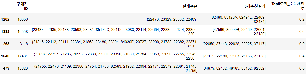
# 추천 시뮬레이션 결과를 살펴보기
k = 5
result_df = simulation_test_df[simulation_test_df['PredictedOrder(Reorder)'].notnull()]
result_df['PredictedOrder(Reorder)'] = result_df['PredictedOrder(Reorder)'].\
                                                        apply(lambda x: x[:k])
result_df = result_df[['CustomerID', 'RealOrdered',
                       'PredictedOrder(Reorder)', 'top_k_recall(Reorder)']]
result_df.columns = [['구매자ID', '실제주문', '5개추천결과', 'Top5추천_주문재현도']]
result_df.sample(5).head()
✔ 딥러닝
개요
- AI > ML(머신러닝) > DL(딥러닝)
- 딥러닝은 여러 비선형 변환 기법의 조합을 통해 노은 수준의 추상화(대량의 데이터 안에서 핵심적이 내용 또는 알고리즘을 요약하는 작업)를 시도하는 머신 러닝 알고리즘 중의 하나
- 데이터가 존재할 때, 컴퓨터가 알아 들을 수 있는 형태로 표현하고 이를 학습에 적용하기 위해 연구된 것 중의 하나
- ANN(퍼셉트론 한개), DNN(퍼셉트론 1개 이상), CNN(합성곱 신경망), RNN(순환 신경망)과 같은 기법들이 존재.
- 일반적으로 머신러닝 알고리즘들은 1~2개의 데이터 표현 층을 이용해서 학습하지만, 딥러닝 모델들은 데이터 표현 층을 무수히 확장해서 학습을 수행함
몇 개의 층으로 이루어진 네트워크
- 원본 데이터를 가지고 다음 층에서 사용할 데이터를 만들고 이런 식으로 각 층에서 사용할 데이터를 만들어 낸 뒤, 가장 마지막에 출력을 생성
- 각각의 층에 어떤 데이터가 들어갈지는 사람이 알아보기가 어려움
작동 원리
- 일련의 숫자로 이루어진 츠으이 가중치를 만들어내는 것
- 이 가중치가 오류가 줄어드는 방향으로 계속 학습
- 첫 가중치는 랜덤하게 생성되고, 그 이후부터는 학습에 의해서 가중치가 수정됨
입력 층(데이터 변환 - 가중치) 층(데이터 변환 - 가중치) ....
- 예측을 하고 실제 값과 비교
- 실제 값과 예측한 결과를 비교하는 함수를 손실 함수(Loss Function)라고 합니다.
- 손실 함수가 만들어 낸 점수를 가지고 옵티마이저를 통과한 뒤, 가중치를 수정해서 다시 학습을 합니다.
- 옵티마이저가 BackPropagation(역전파) 알고리즘을 담당합니다.
특징
- 특성 공학을 자동화 : 전처리가 필요 없음
- 딥러닝의 변환 능력은 순차적으로 동작(Greedily)하지 않고 동시에 공동으로 학습합니다.
- 딥러닝이 각광을 받는 이유는 층을 거치면서 점진적으로 더 복잡한 표현을 만들어내고, 공동으로 학습이 가능하다는 것이다.
발전하게 된 이유
- computing power
- data
- 알고리즘의 발전
- 활성화 함수
- 가중치 초기화 방법
- 배치 정규화
- 잔차 연결
- 합성곱
- 순환 신경망 - Transformer - 대중화
- 초창기에는 C++이나 CUDA를 이용했는데, 지금은 Python 라이브러리(TF, Therno)를 주로 활용
- 단순함 이 중요해짐
- 확장성 : 작은 데이터에서부터 훈련을 해서 확장해 나가는 방식
장점
- 기존 머신러닝보다 성능이 뛰어남
- 특성 엔지니어링에 쏟는 시간을 줄여줌
- 구조화되지 않은 데이털르 가지고 학습이 가능함
단점
- 많은 양의 데이터가 필요함
- 딥러닝에 의해서 학습된 특성들은 해석하기 어려움
- 컴퓨팅 리소스가 많이 필요함
API
- Torch
- C로 구현되어 있고, LuaJIT를 이용해서 개발된 프레임워크 - Theano
- 파이썬으로 만들어진 딥러닝 패키지 - CuDNN
- CUDA를 이용한 딥러닝 패키지 - Tensorflow
- google이 만든 딥러닝 패키지
- 확장성이 좋음
연산
neuron(최근에는 unit이라고 하는 경우가 더 많음)
- 하나 이상의 이진 입력과 하나의 이진 출력으로 구성
perceptron
- 입력과 출력이 이진이 아니라 숫자이고, 각각의 입력 연결은 가중치와 연관되어 있음 (가중치 ==slope)
- Activation Function이라고 하는 출력을 만드는 함수를 이용해서 예측한 값과 실제 값의 차이를 구한 뒤, 이전 차이보다 줄어드는 방향으로 가중치를 수정해 나가면서 학습
- 하나의 perceptron이 일차원 선형 방정식이기 때문에 XOR 문제를 해결할 수 없다.
- 이 문제를 여러 개의 Hidden Layer를 두어서 해결함
- 이것이 Multi Layer Perceptron(MLP) 이다. - 출력의 개수는 회귀의 경우는 무조건 1개이다.
- 분류의 경우는 클래스 개수만큼이 출력의 개수이다.
Activation Function
- 어떤 신호를 받아서 이를 적절히 처리해서 출력해주는 함수
- 선형 활성화 함수
- sign: -1(0보다 작은 경우), 0(0인경우), 1(0보다 큰 경우)
- heviside : 0(0보다 작은 경우), 1(0보다 크거나 같은 경우) - 비선형 활성화 함수
- sigmoid :1/(1+e^(-x)): 입력값이 0 이하면 0.5 이하의 값 출력, 0 이상은 0.5 이상의 값 출력, 딥러닝에서는 역전파(Back Propagation) 알고리즘을 사용하는데, 하나의 층을 통과할 때 마다 가중치가 약해지는데, 이렇게 된다면 Gradient Vanishing(기울기 소멸)현상이 발생함
- softmax : sigmoid를 일반화 한 것으로, 다중 클래스 분류에 사용함
- ReLu
- tanh

밀가루 귀여워요