수업 48일차

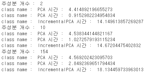
✔ 랜덤 PCA와 점진적 PCA 의 시간 복잡도

# train-images.idx3-ubyte mnist 이미지 데이터 
# 로컬에 있는 데이터를 메모리에 전부 로드된 것 처럼 사용하기
filename='./data/MNIST/raw/train-images.idx3-ubyte'
m,n=X_train.shape
# filename에 데이터를 메모리에 전부 로드한 것 처럼 사용함 - 사용할 때 로드
# 메모리는 한정된 자원인데 메모리 크기보다 
# 훨씬 큰 데이터 가지고 훈련하는 경우에 사용
X_mm=np.memmap(filename, dtype='float32', mode='write', shape=(m,n))
X_mm[:]=X_train
print(m,n)

# 훈련 데이터 가져오기
del X_mm # 변수 지우기 - 메모리 부족시 gc를 호출하는 것을 고려
n_batches=100 # 배치 사이즈는 100
# 52500 //100 = 525개씩 쓰면 되겠네
X_mm=np.memmap(filename, dtype='float32', 
mode='readonly', shape=(m,n))
# 미니 배치의 크기 설정
batch_size=m//n_batches
from sklearn.decomposition import IncrementalPCA #점진적 PCA
inc_pca=IncrementalPCA(n_components=154, batch_size=batch_size)
inc_pca.fit(X_mm) ## 525개씩 메모리에 로드가 된다.
# 일반 PCA는 n_components를 설정할 때,
# 0.0~1.0 사이로 설정하면 분산의 비율이 되고
# 2보다 큰 정수를 설정하면 주성분의 개수가 됩니다.
# RandomPCA는 정수로만 설정합니다.
rnd_pca=PCA(n_components=154, svd_solver='randomized',
random_state=42)
X_reduced=rnd_pca.fit_transform(X_train)

• 시간을 측정해보자.

# 주성분의 개수에 따른 시간 복잡도
import time
for n_components in (2,10,154):
    print("주성분 개수 : ",n_components)
    regular_pca=PCA(n_components=n_components, svd_solver='full')
    rnd_pca=PCA(n_components=n_components,
    svd_solver='randomized', random_state=42)
    inc_pca=IncrementalPCA(n_components=n_components, batch_size=500)
    for pca in (regular_pca, rnd_pca, inc_pca) :
        t1=time.time()# 측정 시작
        pca.fit(X_train)
        t2=time.time()
        print("class name : ", pca.__class__.__name__, 
        "시간 : ", t2-t1)
# inc는 일반적으로 오래 걸리고
# rnd는 컴포넌트 개수에 영향을 받는다.

• 컴포넌트 개수를 늘리면 일반 PCA는 큰 차이가 없지만, rnd_pca가 크게 영향을 받는다.
• inc_pca는 일반적으로 오래 걸리는 것을 확인할 수 있었다.
• 일반적인 수행 속도는 mini batch를 사용하는 IncrementalPCA가 가장 오래 걸리며(전체 트랙잭션을 가지고 Batch Processing을 하는 이유는 실행 시간을 줄이기 위해서)
• RandomizedPCA는 주성분의 근사값을 찾는 알고리즘이므로, 주성분의 개수에 따라 시간 복잡도가 달라진다.
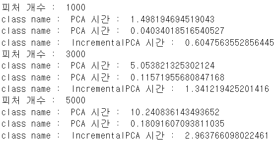
• 일반PCA는 데이터의 개수와 피처의 개수에 영향을 받는다.

# 주성분의 개수에 따른 시간 복잡도
import time
for n_features in (1000,3000,5000):
    print("피처 개수 : ",n_features)
    X=np.random.randn(2000,n_features)
    regular_pca=PCA(n_components=2, svd_solver='full')
    rnd_pca=PCA(n_components=2, svd_solver='randomized',
    random_state=42)
    inc_pca=IncrementalPCA(n_components=2, batch_size=500)
    for pca in (regular_pca, rnd_pca, inc_pca) :
        t1=time.time()# 측정 시작
        pca.fit(X)
        t2=time.time()
        print("class name : ", pca.__class__.__name__, 
        "시간 : ", t2-t1)

• 이번에는 피처의 개수를 바꿔가면서 해보자.
  
• feature 개수가 늘면 시간이 다들 좀 늘긴 하지만, reg_pca가 가장 영향을 많이 받는 것을 확인할 수 있다.

✔ Kernel PCA

Kernel Trick

• 분류나 회귀를 수행할 때, 선형 모양이 아닌 경우에는 고차원으로 매핑해서 회귀나 분류를 수행합니다. (다항식)
• Kernel Trick은 실제로 고차원으로 만드는 것이 아닌, 고차원 공간으로 암묵적으로 매핑해서 비선형 회귀나 분류를 수행하는 기법이다.
• 고차원으로 직접 매핑하게 된다면 시간 복잡도가 급격하게 상승을 합니다.
• PCA에 Kernel Trick을 적용한 것이 Kernel PCA(kPCA)이다.
• decomposition 패키지에서 지원합니다.

매개변수

• Kernel 매개변수에 커널의 종류를 설정
  - linear
  - sigmoid
  - rbf
• rbf의 경우는 gamma를 이용해서 가중치를 설정함
  - 0.0 ~ 1.0 범위
• sigmoid의 경우는 gamma와 coef0를 추가로 설정함
  - gamma를 설정하지 않는다면 0으로 수렴하는 경우가 발생
• fit_inverse_transform에 bool값 설정
  - 복원 가능 여부
  

비지도 학습이라서 성능 측정의 기준이 없지만, 지도 학습의 전처리 단계로 사용되는 경우가 있기 때문에 grid 탐색은 가능합니다.

• 그리드 탐색 가능하다 == 하이퍼 파라미터 튜닝이 가능하다

from sklearn.model_selection import GridSearchCV
from sklearn.linear_model import LogisticRegression
from sklearn.pipeline import Pipeline
from sklearn.decomposition import KernelPCA
from sklearn.datasets import make_swiss_roll
X, t=make_swiss_roll(n_samples=1000, noise=0.2, random_state=42)
# t 는 연속형 수치 데이터라 로지스틱 회귀(분류)에 사용 불가능함
y=t>6.9
clf=Pipeline([
    ('kpca', KernelPCA(n_components=2)),
    ('log_reg', LogisticRegression(solver='lbfgs'))
])
param_grid=[{
    'kpca__gamma':np.linspace(0.03,0.05,10),
    'kpca__kernel':['rbf','sigmoid']
}]
grid_search=GridSearchCV(clf, param_grid,cv=3)
grid_search.fit(X,y)
print(grid_search.best_params_)

• 커널 PCA를 사용하면, 반원이나 동심원 형태로도 주성분 분리가 가능합니다.

✔ PCA 활용

Noise Filtering - 잡음 제거

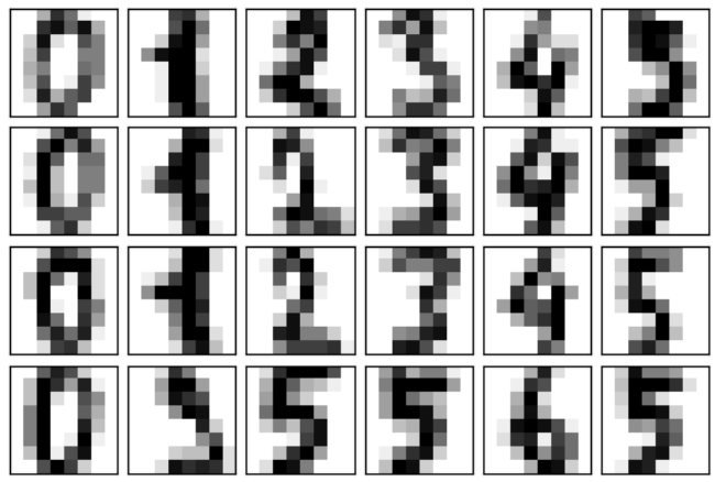
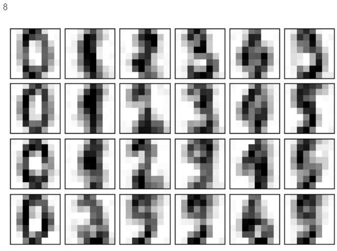
# 숫자 이미지 가져오기
from sklearn.datasets import load_digits
digits=load_digits()
digits.data.shape

• 원본 이미지 확인

def plot_digits(data):
    fig, axes=plt.subplots(4,10,figsize=(10,4),
                           subplot_kw={'xticks':[], 'yticks':[]},
                           gridspec_kw=dict(hspace=0.1,wspace=0.1))
    for i, ax in enumerate(axes.flat):
        ax.imshow(data[i].reshape(8,8),
                 cmap='binary', interpolation='nearest', clim=(0,16))
# 원본 이미지 출력
plot_digits(digits.data)

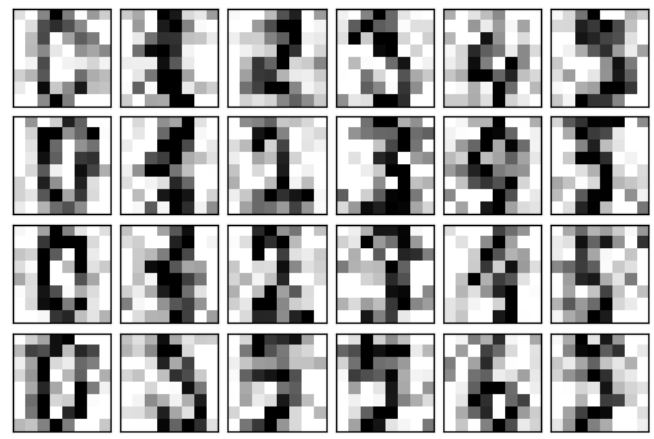
• 노이즈를 넣어보자

# 잡음 추가
np.random.seed(42)
noisy=np.random.normal(digits.data,4)
plot_digits(noisy)

• pca 수행해서 돌려보자.

from sklearn.decomposition import PCA
# PCA를 수행
pca=PCA(n_components=0.4).fit(noisy)
print(pca.n_components_)
components=pca.transform(noisy)
filtered=pca.inverse_transform(components)
plot_digits(filtered)

• 기존 데이터도 같이 조금 유실되겠지만, 복구 완료
• n_components 값을 바꾸면서 작업해보기

✔ 자연어 처리

NLP(National Language Processing) vs Text Analytics

• NLP는 머신이 인간의 언어를 이해하고 해석하는데 중점을 두는 것
• Text Analytics(Text Mining)은 비정형 데이터인 텍스트에서 의미있는 정보를 추출하는 것이다.
• NLP의 영역에서는 언어를 해석하기 위한 기계번역이나 자동으로 질문을 해석하고 답을 해주는 질의응답 시스템 => 'chat bot' 등에 주로 활용함

텍스트 분석의 기술 영역

• 텍스트 분류
  - 텍스트를 보고 어떤 카테고리에 속하는지 분류
• 감성 분석
• 텍스트 요약
  - 대표적인 기법으로 topic modeling
• 텍스트 군집화 & 유사도 측정
• 텍스트 전처리 작업
• ML 모델 수립 및 학습/예측/평가
  - 초창기에는 일반 머신러닝 모델을 가지고 많이 작업을 했는데, 최근에는 DL 의 RNN이나 Transformer와 생성 모델이나 미리 학습된 모델 등을 많이 이용
  

자연어 처리를 위한 패키지

• NLTK
  - 가장 많이 사용되던 자연어 처리 패키지
  - 최근에는 거의 학습용으로만
  - 수행 속도가 느려 대량 텍스트 기반 자연어 처리에는 부적합
• Gensim
  - 토픽 모델링에서 많이 사용되는 패키지
  - word2vec 같은 알고리즘이 구현되어 있습니다.
• SpaCy
• Konlpy
  - 한글 형태소 분석 패키지

그 이외 Tensorflow나 Pytorch 또는 사전학습 모델인 Bert, CHATGPT같은 모델을 많이 이용합니다.

한글 형태소 분석기 설치

• 1.7 버전 이상의 JDK 설치하고 PATH에 JDK 경로의 bin 추가하고, JAVA_HOME이라는 환경변수에 JDK의 경로를 추가해야 한다.
• JPype1-py3를 설치하자
• pip 되는 경우가 있고 안된다면 conda로 하면 된다.
• 이후 konlpy 설치

텍스트 전처리

• 텍스트 자체를 바로 feature로 사용할 수 없기 때문에, 사전에 특스트를 가공하는 작업이 필요합니다.

전처리 작업

• 클렌징
  - 불필요한 문자열 제거
• 토큰화
  - 단어나 글자를 분리
• 필터링
  - 스톱워드 제거, 철자 수정
• Stemming & Lemmatization

토큰화

• 문장 토큰화나 단어 토큰화 2가지
• 문장 토큰화
  - 마침표나 개행문자 (\n or \r\n)를 기준으로 문장을 분리하는 것
  - 정규 표현식을 이용하기도 합니다.
  - nltk 패키지의 punkt 서브 패키지 이용
  - sent_tokenize 함수를 사용합니다.
  

# nltk 패키지의 punkt 서브 패키지 설치
import nltk
nltk.download('punkt')

# 문장 토큰화
text_sample='hello world! nicki minaj. jessie j. ariana grande'
from nltk import sent_tokenize
sentences=sent_tokenize(text_sample)
print(sentences)

• 단어 토큰화
  - 문장을 단어로 토큰화 하는 것
  - 공백, 콤마, 개행 문자 단위로 토큰화
  - nltk 패키지의 word_tokenize함수를 이용합니다.

# 단어 토큰화
t= '손으로 코딩하고 뇌로 컴파일하며 눈으로 디버깅하자 \n 집에 가고싶다'
from nltk import word_tokenize
words=word_tokenize(t)
print(words)

Stop Word 제거

• Stop Word(불용어)
  - 분석에 큰 의미가 없는 단어
  - 영어의 경우는 nltk 패키지에서 제공합니다.
  - 패키지에서 제공하는 것 만으로는 충분하지 않기에 직접 추가해서 사용하는 경우가 많다.

import nltk
nltk.download('stopwords')
print('불용어 개수 : ', len(nltk.corpus.stopwords.words('english')))
print('불용어 : ',nltk.corpus.stopwords.words('english') )
stopwords=nltk.corpus.stopwords.words('english')
print(type(stopwords)) # list 타입이다
# 직접 추가도 가능하다.
stopwords.append('jessie')
print('불용어 개수 : ', len(stopwords))

from nltk import sent_tokenize
# 문장 토큰화
text_sample='hello world! I am a big fan of nicki minaj.
jessie j. ariana grande'
sentences=sent_tokenize(text_sample)
wordtokens=[word_tokenize(sentence) for sentence in sentences]
all_tokens=[]
for sentence in wordtokens:
    filtered_words=[]
    for word in sentence :
        # 영문의 경우는 대소무자 
        word=word.lower()
        if word not in stopwords:
            filtered_words.append(word)
    all_tokens.append(filtered_words)
print(all_tokens)

Stemming과 Lemmatization

• 동일한 단어가 과거나 현재 또는 복수와 단수 그리고 진행형 등 많은 조건에 따라 단어가 변경된다.
• 동일한 의미를 가지고 있는 단어의 어근을 찾아서 사용해야 하는 경우가 발생함
• 단어의 어근을 찾아주는 API로 Stemming과 Lemmatization이 제공됨
• Stemming은 원형 단어로 변환할 때 일반적인 적용을 하거나, 더 단순화된 방법을 적용해서 원래 단어에서 일부 철자가 훼손된 어근 단어를 추출하는 경향이 있음
• Lemmatization은 품사와 같은 문법적인 요소와 더 의미적인 부분을 감안해서 어근을 찾아주기에 더 정교함
• NLTK에서는 Stemmer를 위해서 Porter, Lancaster, Snowball Stemmer를 제공하고, Lemmatization을 위해서는 WordNetLemmatization을 제공합니다.

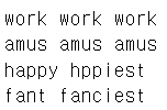
from nltk.stem import LancasterStemmer
stemmer=LancasterStemmer()
print(stemmer.stem('working'),stemmer.stem('works'),
stemmer.stem('worked'))
print(stemmer.stem('amusing'),stemmer.stem('amuses'),
stemmer.stem('amused'))
print(stemmer.stem('happy'),stemmer.stem('hppiest'))
print(stemmer.stem('fancier'),stemmer.stem('fanciest'))

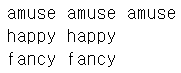
import nltk
nltk.download('omw-1.4')

from nltk.stem import WordNetLemmatizer
import nltk
nltk.download('wordnet')
lemma = WordNetLemmatizer()
print(lemma.lemmatize('amusing','v'),
lemma.lemmatize('amuses','v'),lemma.lemmatize('amused','v'))
print(lemma.lemmatize('happier','a'),
lemma.lemmatize('happiest','a'))
print(lemma.lemmatize('fancier','a'),
lemma.lemmatize('fanciest','a'))

텍스트 피처화 - BoW

• Bag of Words의 약자로, 문서가 가지는 모든 단어를 문맥이나 순서를 무시하고 일괄적으로 단어에 대해 빈도 값을 부여해서 피처 값을 추출하는 모델
• My wife likes to watch baseball games and my daughter likes to watch baseball games too.
• My wife likes to play baseball
• 위의 문장에서 중복을 제거한 모든 단어를 추출
• 장점
  - 쉽고 빠른 구축
• 단점
  - 문맥의 의미 반영을 안함
  - 단어의 순서를 고려하지 않음
  - 실제 여러 개의 문장이 존재한다면, 각 단어는 문장에 포함되지 않을 가능성이 높기 때문에, 0이 아주 많아지게 되고, 이렇게 0이 많으면 대다수의 경우에는 희소 행렬(Sparse Matrix)로 표현하게 되는데, 희소행렬은 대다수의 ML 알고리즘의 성능을 떨어뜨립니다.
  

BoW Feature 벡터화

• 숫자의 배열로 변환
• 카운트 기반의 벡터화
  - 단어 피처에 값을 부여할 때, 각 문서에서 단어가 등장한 횟수를 부여
  - wordcloud에서 주로 이용
• TD-IDF(Term Frequency - Inverse Document Frequency) 기반의 벡터화
  - 개별 문서에서 자주 등장하는 단어에는 가중치를 부여하고, 여러 문서에서 자주 등장하는 단어는 패널티를 부여하는 방식
  - 가중치=개별 문서에서의 빈도* (log(문서의 개수/ 단어를 갖고 있는 문서 개수))

희소 행렬 표현 방식

• COO 형식
  - 0이 아닌 데이터만 별도의 배열에 저장하고, 그 데이터가 가리키는 행과 열의 위치를 별도의 배열에 저장하는 방식

[[3 0 1][0 2 0]]

• 0이 아닌 곳은 3과 1과 2 : [3 1 2]
• 위치를 배열로 생성 : [[0 0 1],[0 2 1]]
• scipy의 sparse 패키지에 이러한 변환을 위한 함수를 소유하고 있음
• coo_matrix 함수가 이 역할을 수행하고, toarray()를 호출하면 밀집 배열로 변환할 수 있습니다.

data=np.array([3,1,2])
row_pos=np.array([0,0,1])
col_pos=np.array([0,2,1])
from scipy import sparse
sparse_coo=sparse.coo_matrix((data,(row_pos,col_pos)))
print(sparse_coo)

• CSR 형식
  - 데이터 배열은 동일한데, COO 방식에서 동일한 인덱스를 여러 번 반복하는 것을 방지하는 방식
  - 행의 인덱스가 앞에서 [0 0 1 1 1 1 2 2 3 4 4 5] 로 있는 경우행의 인덱스는 순차적으로 진행하는데, 이런 경우, 0이 2개 1이 4개 2가 2개 3 1개 4 2개 5 1개 이다.
  - 이런 경우, 중복 데이터를 2번 기재하지 않고, 시작하는 위치만 기록
  - [0 2 6 8 9 11] 이런 형태로 시작 위치만 표시합니다.

dense_matrix=np.array([[0,0,1,0,0,5], [1,4,0,3,2,5],
                       [0,6,0,6,0,0],[2,0,0,0,0,0],
                      [0,0,0,7,0,8],[1,0,0,0,0,0]])
data=np.array([1,5,1,4,3,2,5,6,6,2,7,8,1])
row_pos=np.array([0,0,1,1,1,1,1,2,2,3,4,4,5])
row_pos_index=np.array([0,2,7,9,10,12,13])
col_pos=np.array([2,5,0,1,3,4,5,1,3,0,3,5,0])
sparse_csr=sparse.csr_matrix((data,col_pos,row_pos_index))
print(sparse_csr.toarray())

sklearn의 BoW Feature 벡터와 클래스

• CountVectorizer 클래스
  - 카운트 기반의 벡터화를 구현한 클래스
  - 소문자 일괄 변환, 토큰화 그리고 스톱 워드 필터링 기능도 제공함
  - fit과 transform 메서드를 이용해서 변환을 수행합니다.
• 입력 파라미터
  - max_df : 너무 높은 빈도수의 단어를 제외하기 위한 옵션
  - min_df : 너무 낮은 빈도수의 단어를 제외하기 위한 옵션
  - max_features : 추출하는 피처의 개수를 제한
  - stop_words : 불용어
  - n_gram_range : 단어의 순서를 어느 정도 보장하기 위해 max,min을 tuple 형태로 설정해서 순서를 지킬 범위를 설정함
  - analyzer : 피처 추출을 위한 단위를 설정하는 것. 기본은 단어, 단어 내에서의 글자 범위 설정 가능(몇글자..)
  - token_pattern : 토큰화를 수행하는 정규 표현식을 설정
  - tokenizer : 토큰화를 별도의 함수를 이용해서 수행하고자 하는 경우, 함수에 대한 포인터 설정

Word Cloud

• word cloud 또는 Tag Cloud라고도 합니다.
• 단어의 중요도나 인기도를 고려해서 시각적으로 늘어놓아 표시
• tag cloud나 wordcloud 패키지 설치

TagCloud 패키지 이용

• 패키지 설치
  - pytagcloud
  - pygame
  - simplejson
  

작업 순서

• 단어의 리스트 생성
• Collections 모듈의 Counter를 이용해서 각 단어의 개수를 가지는 Counter 객체를 생성
• Counter 객체의 most_commons(사용할 데이터 개수)를 호출해서 단어와 단어 별 개수를 튜플로 갖는 list를 생성
• pytagcloud.make_tags(태그 목록, maxsize=최대크기)
• pytagcloud.create_tag_image(앞에서 만들어진 결과, 이미지 파일 경로, fontname='한국어를 출력하고자 하는경우', rectangular=사각형여부)
• 한글 폰트를 사용하고자 하는 경우
  - 폰트 파일을 pytagcloud가 설치된 곳의 fonts 디렉토리에 복사를 수행합니다.
  - font.json 파일에 폰트를 등록해야 합니다.
  [{'name':'폰트이름','ttf':'폰트 파일 경로','web':'웹 글꼴경로}]
  - windows에서는 아나콘다 설치 디렉\lib\site-package\pytagcloud일 것이다.
  - 아니면 USER\AppData\Local\Programs\Python\Python38\Lib\site-packages\ 일 것이다.
  - NanumBarunGothic.ttf써보자.

한글 태그 클라우드 작성

• 사용할 폰트를 pytagcloud/fonts 디렉토리에 복사하기
• fonts.json 에서 json 형식으로 정보 추가해주기

{
		"name": "Korean",
		"ttf": "NanumBarunGothic.ttf",
		"web": "http://fonts.googleapis.com/css?famliy=Nobile"
}

• 그냥 데이터 왕창 생성하기

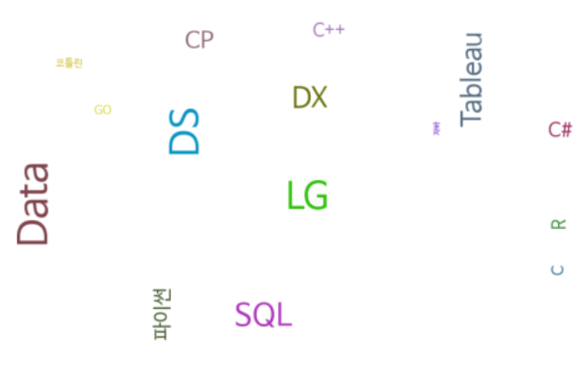
import pytagcloud
import collections
nouns=[]
nouns.extend(['파이썬' for t in range(8)])
nouns.extend(['자바' for t in range(2)])
nouns.extend(['GO' for t in range(4)])
nouns.extend(['코틀린' for t in range(3)])
nouns.extend(['R' for t in range(7)])
nouns.extend(['Tableau' for t in range(12)])
nouns.extend(['SQL' for t in range(15)])
nouns.extend(['C' for t in range(6)])
nouns.extend(['C++' for t in range(7)])
nouns.extend(['C#' for t in range(8)])
nouns.extend(['Data' for t in range(21)])
nouns.extend(['DS' for t in range(20)])
nouns.extend(['DX' for t in range(13)])
nouns.extend(['LG' for t in range(18)])
nouns.extend(['CP' for t in range(10)])
print(nouns)

# 데이터 개수 세기 - list에서 데이터 개수 세기
count=collections.Counter(nouns)
# print(type(count))
# print(dir(count))
# print(count)
'''
# __iter__가 있다면 순회가 가능하다
for x in count:
    print(x, count[x])
'''
# 가장 많이 등장한 것의 개수를 설정해서 가져오기
tag=count.most_common(15)
print(tag)
# 태그 목록 만들기
taglist=pytagcloud.make_tags(tag,maxsize=50)
print(taglist)
# 태그 클라우드 생성
pytagcloud.create_tag_image(taglist,'wordcloud.png',
                           size=(900,600), fontname="Korean",
                            rectangular=False)
img=mpl.image.imread('wordcloud.png')
imgplot=plt.imshow(img)
plt.axis('off')
plt.show()

• 완성!

wordcloud 패키지는 뭘 할 수 있을까

• 이미지를 먼저 배경으로 만들고 이미지 위에 워드클라우드를 작성할 수 있음
• pip install wordcloud

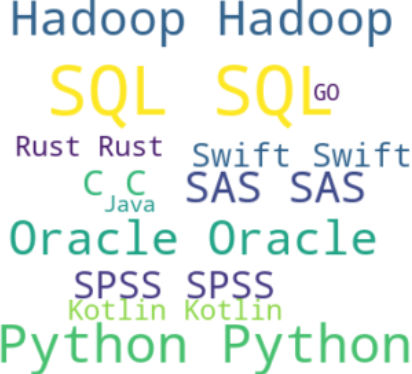
from PIL import Image
mask=np.array(Image.open('./data/star.png'))
plt.figure(figsize=(8,8))
plt.imshow(mask, cmap=plt.cm.gray, interpolation='bilinear')

# 문자열 만들기
text=''
for i in range(18):
    text=text+'Python '
for i in range(5):
    text=text+'C '
for i in range(3):
    text=text+'Java '
for i in range(20):
    text=text+'SQL '
for i in range(16):
    text=text+'R '
for i in range(12):
    text=text+'SAS '
for i in range(9):
    text=text+'SPSS '
for i in range(4):
    text=text+'C++ '
for i in range(3):
    text=text+'GO '
for i in range(6):
    text=text+'Kotlin '
for i in range(7):
    text=text+'Swift '
for i in range(6):
    text=text+'Rust '
for i in range(5):
    text=text+'Ruby '
for i in range(14):
    text=text+'Oracle '
for i in range(15):
    text=text+'Hadoop '
print(text)

• 불용어 처리

from wordcloud import WordCloud, STOPWORDS
stopwords=set(STOPWORDS)
stopwords.add('Ruby')

wordcloud=WordCloud(background_color='white', max_words=2000,
                   mask=mask, stopwords=stopwords)
wordcloud=wordcloud.generate(text)
# wordcloud.words_
plt.figure(figsize=(12,12))
plt.imshow(wordcloud, interpolation='bilinear')
plt.axis('off')
plt.show()

• 단어가 중복되어서 나오는게 싫다!

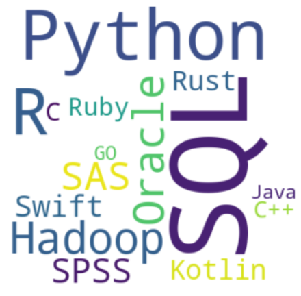
# 단어 빈도수 계산
word_frequencies = {}
words = text.split()
for word in words:
    if word in word_frequencies:
        word_frequencies[word] += 1
    else:
        word_frequencies[word] = 1

• 이거를 텍스트 만들고 넣어주고

wordcloud=WordCloud(background_color='white', max_words=2000,
                   mask=mask, stopwords=stopwords)
wordcloud = wordcloud.generate_from_frequencies(word_frequencies)

• 이렇게 처리해주자
  
• 짠

동아일보에서 뉴스를 검색해서 크롤링 한 뒤, 워드 클라우드 생성

• 정적 텍스트는 BS4 있으면 크롤링해서 사용 가능
• 동적 텍스트(로그인, ajax 등..)를 읽어오는 경우에는 Selenium같은 별도의 패키지를 활용해야 합니다.

크롤링을 할 때는 url 패턴을 좀 알아야 합니다.

• url에서 파라미터 부분(?다음부분)은 반드시 인코딩이 되어야 합니다.
• 일본을 검색했을 때,
  - https://www.donga.com/news/search?query=%EC%9D%BC%EB%B3%B8 이다.
• 더보기, 페이지 번호 등도 다 확인해야 합니다. 이것들이 다 url입니다.
• https://www.donga.com/news/search?query=%EC%9D%BC%EB%B3%B8&sorting=1&check_news=91&search_date=1&v1=&v2=&more=1 -더보기
• https://www.donga.com/news/search?p=16&query=%EC%9D%BC%EB%B3%B8&check_news=91&more=1&sorting=1&search_date=1&v1=&v2= -2페이지
• 여기서는 p 파라미터랑 query파라미터가 중요하다.
• p : 기사 일련번호, 1부터 시작, 증가 단위 15
• query : 검색어

실습 시작

# Web의 정적 컨텐츠를 다운로드 받기 위한 패키지
import requests
from urllib.parse import quote
# html 파싱을 위한 패키지
from bs4 import BeautifulSoup
keyword=input('검색어 : ')
target_URL="https://www.donga.com/news/search?query="+quote(keyword)+"&sorting=1&check_news=91&search_date=1&v1=&v2=&more=1"
source_code=requests.get(target_URL)
# print(target_URL)
# print(source_code)
# print(source_code.text)
# html 파싱 객체 생성
bs=BeautifulSoup(source_code.text, 'html.parser')
# 파싱
tags=bs.select('div.cntPage > span') 
# 선택자는 중복이 가능하기에 list로 리턴하자
count=int(tags[0].getText()[0:-1].replace(',',''))
print('기사 건수 : ',count)

# 실제로 크롤링 할 기사 건수 입력 받기
read_cnt=int(input("읽을 기사 건수:"))
if read_cnt>count:
    read_cnt=count
# 읽을 페이지 개수
page_num=int(read_cnt/15+0.95)
print(page_num)

data = []
# 다운로드 받은 텍스트를 저장할 파일을 개방
output_file=open(keyword+'.txt','w',encoding='utf8')
#content > div.sch_cont > div.schcont_wrap > div > div:nth-child(2) > div.rightList > span.tit > a
for i in range(page_num):
    current_p = 1 + i * 15
    target_URL = "https://www.donga.com/news/search?p="+str(current_p)+"&query="+quote(keyword)+"&check_news=91&more=1&sorting=1&search_date=1&v1=&v2="
    # 페이지 순회가 가능한 각 검색 페이지의 데이터를 가져옵니다.
    source_code = requests.get(target_URL)
    print(source_code)
    # 각 페이지의 데이터를 파싱합니다.
    bs = BeautifulSoup(source_code.text, 'html.parser')
    page_links = []
    # 각 페이지에서 기사 링크를 찾습니다.
    for j in range(2, 17):
        page_links.append(bs.select('div:nth-child(' + str(j) + ') > div.rightList > span.tit > a'))
    for link_list in page_links:
        for link in link_list:
            title_link = link['href']
            source_code = requests.get(title_link)
            bs = BeautifulSoup(source_code.text, 'html.parser')
            # 원하는 부분(텍스트)만 크롤링하여 출력하거나 data 리스트에 추가합니다.
            articles = bs.select('#article_body')
            if articles is not None:
                for article in articles:
                    # 데이터를 출력하거나 data 리스트에 추가하는 부분을 여기에 추가하세요.
                    # 예를 들어, 출력하려면 print(article.getText())를 사용할 수 있습니다.
                    data.append(article.getText())
                    string_item=str(article.find_all(text=True))
                    output_file.write(string_item)
output_file.close()

• 이제 워드클라우드 준비

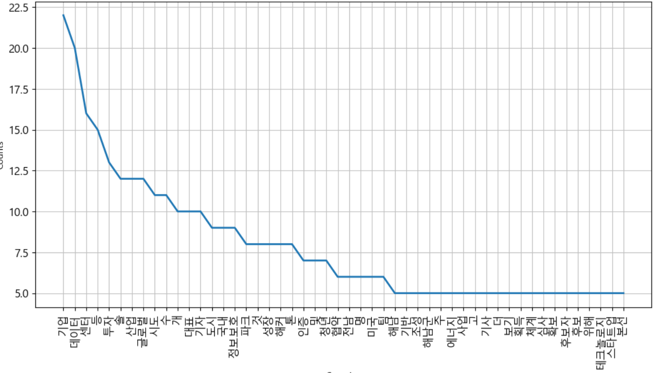
# 한글 형태소 분석기를 활용해서 한글 텍스트를 추출하자
from konlpy.tag import Twitter
open_text_file=open(keyword+'.txt', 'r', encoding='utf8')
text=open_text_file.read()
spliter=Twitter()
nouns=spliter.nouns(text)
open_text_file.close()
print(nouns)

# 단어 개수와 등장 횟수 확인
import nltk
ko=nltk.Text(nouns, name=keyword)
print('전체 단어 개수 : ', len(ko.tokens))
print('전체 단어 개수 - 중복 제거 : ', len(set(ko.tokens)))
# print(dir(ko.vocab()))
plt.figure(figsize=(12,6))
ko.plot(50)
plt.show()

• 한글자는 지우는게 나을 것 같아.

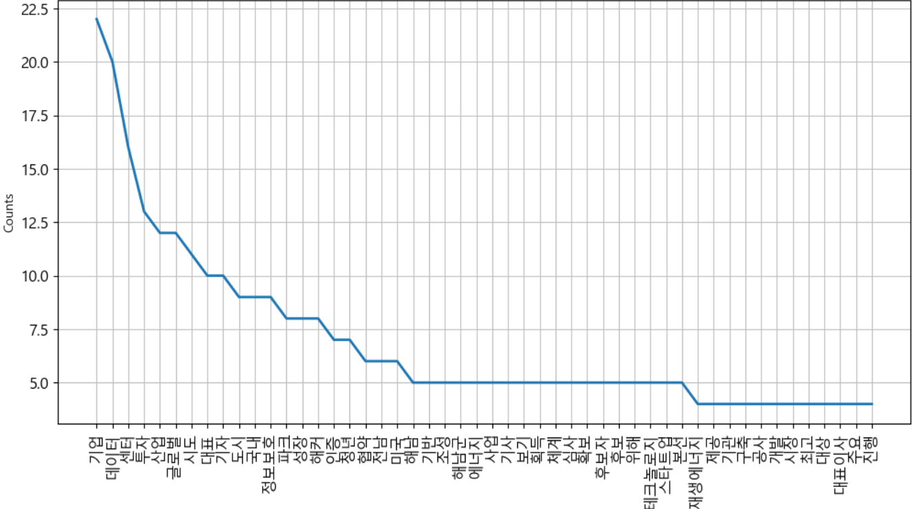
# 불용어 제거
stop_words=[]
# list comprehension이 일반적으로 파이썬에서 가장 빠르다
ko_1=[each_word for each_word in ko if each_word not in stop_words]
ko_2=[each_word for each_word in ko_1 if len(each_word)>1]
ko=nltk.Text(ko_2, name=keyword)
plt.figure(figsize=(12,6))
ko.plot(50)
plt.show()

• 이제 만들자

# 워드 클라우드 생성
mask=np.array(Image.open('./data/apple.png'))
data=ko.vocab().most_common(150)
wordcloud=WordCloud(relative_scaling=0.5,font_path='./data/NanumBarunGothic.ttf',
                    mask=mask,
                   background_color='white').generate_from_frequencies(dict(data))
plt.figure(figsize=(12,6))
plt.imshow(wordcloud)
plt.axis('off')
plt.show()

• 진짜 끝

텍스트 분류

• sklearn에서는 fetch_20newsgroups라는 API를 이용해서 뉴스 그룹의 분류를 수행해 볼 수 있는 예제(데이터)를 제공합니다.
• 텍스트를 feature 벡터화하면 일반적으로 희소 행렬 형태가 되고, 이러한 희소 행렬의 데이터를 가지고 분류를 잘 하는 알고리즘은 로지스틱 회귀, SVM, 나이브 베이즈 등..
• 텍스트를 가지고 분류를 할 때는 먼저 텍스트를 정규화(전처리)를 수행하고 피처 벡터화를 하고 그 이후에 머신 러닝 알고리즘을 적용

뉴스 그룹 분류

# 데이터 가져오기
from sklearn.datasets import fetch_20newsgroups
news_data=fetch_20newsgroups(subset='all', random_state=42)
print(news_data.keys())

# 인덱스 소트해서 카운팅
print(pd.Series(news_data.target).value_counts().sort_index())
# 타겟 이름 확인
print(news_data.target_names)
#데이터 확인
print(news_data.data[0])

• 데이터를 확인해보면 기사 내용 뿐만 아니라, 제목, 작성자 소속 이메일 등이 포함되어 있어서 이부분은 제거를 하고 사용해야 할 것 같다.
• 이 경우는 데이터 가져올 때, remove 옵션에 headers footers quotes 를 설정하면 텍스트만 넘어옵니다.