선형회귀 분석
필수라이브러리 설치 및 모델링 전 사전 작업
* 라이브러리 설치
* 원핫인코딩을 위해 category_encoders 라이브러리를 설치해줍니다.
!pip install category_encoders
* for Ridge, Lasso normalize=True options
해당 라이브러리 설치 후 런타임 다시 시작 -> 이후 셀 진행
!pip install scikit-learn==1.1.3
* 사용할 라이브러리 추가
import numpy as np
import pandas as pd
import matplotlib.pyplot as plt
import seaborn as sns
import warnings
from sklearn.preprocessing import StandardScaler, PolynomialFeatures
from sklearn.linear_model import LinearRegression, Ridge, Lasso
from sklearn.preprocessing import LabelEncoder
from sklearn.model_selection import train_test_split
from sklearn.preprocessing import StandardScaler
from sklearn.metrics import r2_score, mean_absolute_error
from sklearn.model_selection import cross_val_score
from sklearn.linear_model import Ridge
from sklearn.linear_model import Lasso
from sklearn.feature_selection import f_regression, SelectKBest
from sklearn.metrics import mean_absolute_error, mean_squared_error
warnings.filterwarnings(action='ignore')
* 데이터셋 가져오기
naver_shop = pd.read_csv('https://raw.githubusercontent.com/yskim1230/AIB_Section2-PJT_Modeling-Plan/main/naver_shop_FE_comp.csv')
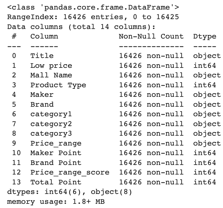
naver_shop.info()

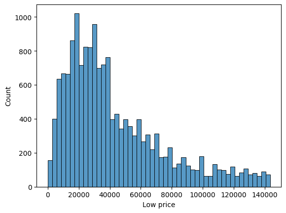
* 타겟 분포 확인
sns.histplot(naver_shop['Low price'], bins=50);
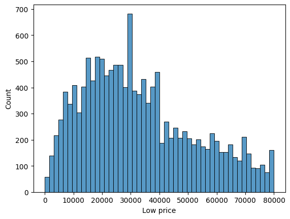
* 'Low price' 값이 100,000보다 작은 데이터만 추출하여 'naver_shop_cl' 데이터프레임 생성
naver_shop_cl = naver_shop[naver_shop['Low price'] < 80000]
* 'Low price' 컬럼의 히스토그램 그리기
sns.histplot(naver_shop_cl['Low price'], bins=50);
* 데이터 금액 구간을 나눠 4분류로 했을때
* 'Price_range' 컬럼을 범주형 변수로 변환
naver_shop['Price_range'] = pd.Categorical(naver_shop['Price_range'], categories=['Very Cheap', 'Cheap', 'Moderate', 'Expensive'], ordered=True)

* 'Price_range' 변수의 분포 확인
sns.countplot(x='Price_range', data=naver_shop)
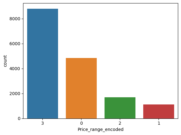
* 'Price_range' 컬럼을 라벨 인코딩하여 'Price_range_encoded' 변수에 저장
encoder = LabelEncoder()
encoder.fit(['Very Cheap', 'Cheap', 'Moderate', 'Expensive']) # 순서 지정
naver_shop = naver_shop.dropna(subset=['Price_range'])
naver_shop['Price_range_encoded'] = encoder.transform(naver_shop['Price_range'])
order = naver_shop['Price_range_encoded'].value_counts().index.tolist()
sns.countplot(x='Price_range_encoded', data=naver_shop, order=order)
'Product Type'과 'Low price' 간의 상관계수 구하기
corr = naver_shop[['Product Type', 'Low price']].corr()
상관도 히트맵 그리기
sns.heatmap(corr, annot=True, cmap='YlGnBu')
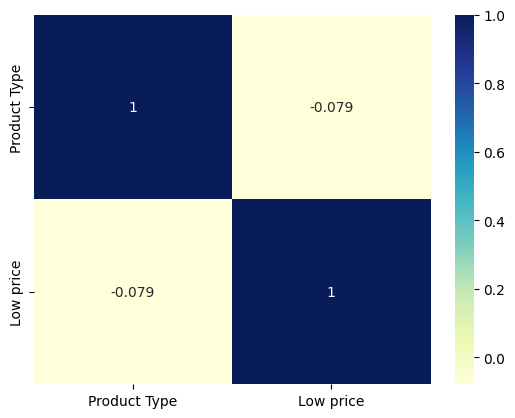
음의 상관계수가 나왔으나 int형이 product type밖에 인식되지 않았다.
모델링
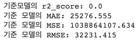
1. 기준모델
* 기준모델 생성
baseline = [y_train.mean()] * len(y_train)
baseline_r2 = r2_score(y_train, baseline)
baseline_mae = mean_absolute_error(y_train, baseline)
baseline_mse = mean_squared_error(y_train, baseline)
baseline_rmse = np.sqrt(baseline_mse)
* 결과 출력
print(f'기준모델의 r2_score: {baseline_r2}')
print(f"기준 모델의 MAE: {baseline_mae:.3f}")
print(f"기준 모델의 MSE: {baseline_mse:.3f}")
print(f"기준 모델의 RMSE: {baseline_rmse:.3f}")
2. 다항선형회귀
* 독립 변수와 타겟 변수 선택
X_cols = ['Maker Point', 'Brand Point', 'Price_range_score','Total Point']
y_col = 'Low price'
X = naver_shop[X_cols]
y = naver_shop[y_col]
* 데이터 정규화
scaler = StandardScaler()
X_scaled = scaler.fit_transform(X)
* train 데이터와 test 데이터로 분할
X_train, X_test, y_train, y_test = train_test_split(X_scaled, y, test_size=0.2, random_state=42)
* train, test 데이터가 잘 나눠졌는지 확인.
X_train.shape, X_test.shape, y_train.shape, y_test.shape

* 선형회귀 모델 만들기
ols = LinearRegression()
* 모델 학습
ols.fit(X_train, y_train)
* 성능 평가
train_score = np.round(ols.score(X_train, y_train), 3)
val_score = np.round(np.mean(cross_val_score(ols, X_train, y_train, scoring='r2', cv=3)), 3)
test_score = np.round(ols.score(X_test, y_test), 3)
* 모델 예측
y_pred = ols.predict(X_test)
* MAE, MSE, RMSE, R^2 계산
mae = mean_absolute_error(y_test, y_pred)
mse = mean_squared_error(y_test, y_pred)
rmse = np.sqrt(mse)
r2 = r2_score(y_test, y_pred)
* 결과 출력
print(f"R^2: {r2:.3f}")
print(f"MAE: {mae:.3f}")
print(f"MSE: {mse:.3f}")
print(f"RMSE: {rmse:.3f}")
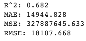
기존 모델 보다 개선
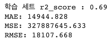
3. One-hot-encoding(category3)
* category3 변수에 대해 one-hot encoding을 수행
category3_encoded = pd.get_dummies(naver_shop['category3'], prefix='category3')
* 인코딩된 데이터를 원본 데이터에 병합
naver_shop = pd.concat([naver_shop, category3_encoded], axis=1)
* 독립 변수와 타겟 변수 선택
X_cols_ohe = ['Maker Point', 'Brand Point', 'Price_range_score'] + list(category3_encoded.columns)
y_col_ohe = 'Low price'
X_ohe = naver_shop[X_cols_ohe]
y_ohe = naver_shop[y_col_ohe]
* 데이터 정규화
scaler_ohe = StandardScaler()
X_scaled_ohe = scaler.fit_transform(X)
* train 데이터와 test 데이터로 분할
X_train_ohe, X_test_ohe, y_train_ohe, y_test_ohe = train_test_split(X_scaled_ohe, y_ohe, test_size=0.2, random_state=42)
* 선형회귀 모델 만들기
ols = LinearRegression()
* 모델 학습
ols.fit(X_train_ohe, y_train_ohe)
* 성능 평가
train_score_ohe = np.round(ols.score(X_train_ohe, y_train_ohe), 3)
val_score_ohe = np.round(np.mean(cross_val_score(ols, X_train_ohe, y_train_ohe, scoring='r2', cv=3)), 3)
test_score_ohe = np.round(ols.score(X_test_ohe, y_test_ohe), 3)
* 결과 출력
print(f'학습 세트 r2_score : {train_score_ohe}')
모델 예측
y_pred = ols.predict(X_test_ohe)
* MAE, MSE, RMSE 계산
mae_ohe = mean_absolute_error(y_test_ohe, y_pred)
mse_ohe = mean_squared_error(y_test_ohe, y_pred)
rmse_ohe = np.sqrt(mse_ohe)
* 결과 출력
print(f"MAE: {mae_ohe:.3f}")
print(f"MSE: {mse_ohe:.3f}")
print(f"RMSE: {rmse_ohe:.3f}")
선형회귀 모델 해석
두 모델 다 기준 모델 대비 R^2 score가 증가하고, MAE가 감소하며 MSE, RMSE가 모두 감소한다면, 이는 새로운 모델이 기준 모델보다 더 나은 예측 성능을 보인다는 것을 의미.
R^2 score가 증가하면 모델이 종속 변수의 분산을 더 잘 설명하는 것이므로, 예측 성능이 개선되었다는 것을 나타냅니다. MAE가 감소하면 모델의 예측값과 실제 값 간의 차이가 작아졌으므로 예측 성능이 개선되었다는 것을 의미합니다. MSE와 RMSE가 감소하면 모델의 예측 오차가 더 작아졌다는 것을 의미합니다.
다만 다항선형회귀와 one-hot-encoding을 사용하여 타겟 변수에 차이를 둔 2개 모델링에서는
r^2 Score는 아주 미세하게 개선되었으나
MAE, MSE, RMSE가 같다.
R^2 score가 미세하게 개선되었지만, MAE, MSE, RMSE가 동일하게 유지된다면, 모델의 예측 성능이 크게 개선되지 않았음을 의미한다.