EBCLR

Contrastive learning은 Deep Neural Networks (DNNs)를 훈련함으로써 visual representation을 학습하는 방법이다. 일반적으로 positive pairs (transformations of the same image)들의 유사도는 증가시키고 negative pairs (transformations of different images)들의 유사도는 감소시킨다.

이 논문에서는 EBM(Energy-based Models)과 contrastive learning을 결합하여 the power of generative learning을 활용한다. EBCLR은 이론적으로 joint distribution of positive pairs를 학습하는 것으로 해석할 수 있고, MNIST, Fashion MNIST, CIFAR-10 및 CIFAR100과 같은 중소 규모 데이터 셋에서 좋은 결과를 얻는다.

---

EBM에 대해 모르는 사람이라면, Energy-based Model이 가지고 있는 power of generative learning이라는 뜻의 의미를 제대로 해석하기가 어렵다. Energy-based model을 아주 간단하게 설명해보면, 어떤 에너지 함수를 통해 두 변수 X,Y를 scalar로 매핑하는 모델이며, 이 때 옳은 페어인 (X,Y)에 대해서 에너지 값이 낮아지도록 model을 만들어 낸다고 생각하면 될 것이다. 마치 머신러닝 모델이 어떤 입력을 받아 모든 y의 logits값중에 가장 높은 값이 정답 class라고 예측하듯, EBM은 어떤 입력 joint distribution $p(x,y)$ 혹은 $p(x)$에 대한 옳은 정답을 내뱉도록 하는 모델링 방법이라고 이해하면 되지 않을까 싶다.

---

특히, EBCLR은 SimCLR과 MoCo v2에 비해 4배에서 20배의 가속도를 보인다.

더불어, 하나의 positive pair당 254개의 negative pairs(batch 256)로 훈련된 SimCLR과 비교하여 30개의 negative pairs(batch 32)로 거의 동일한 성능을 달성하여 적은 수의 네거티브 페어에 대한 EBCLR의 우수성을 입증했다. EBCLR은 합리적인 성능을 달성하기 위해 다른 방법들에 비해 적은 수의 negative pair가 필요한 방법이다.

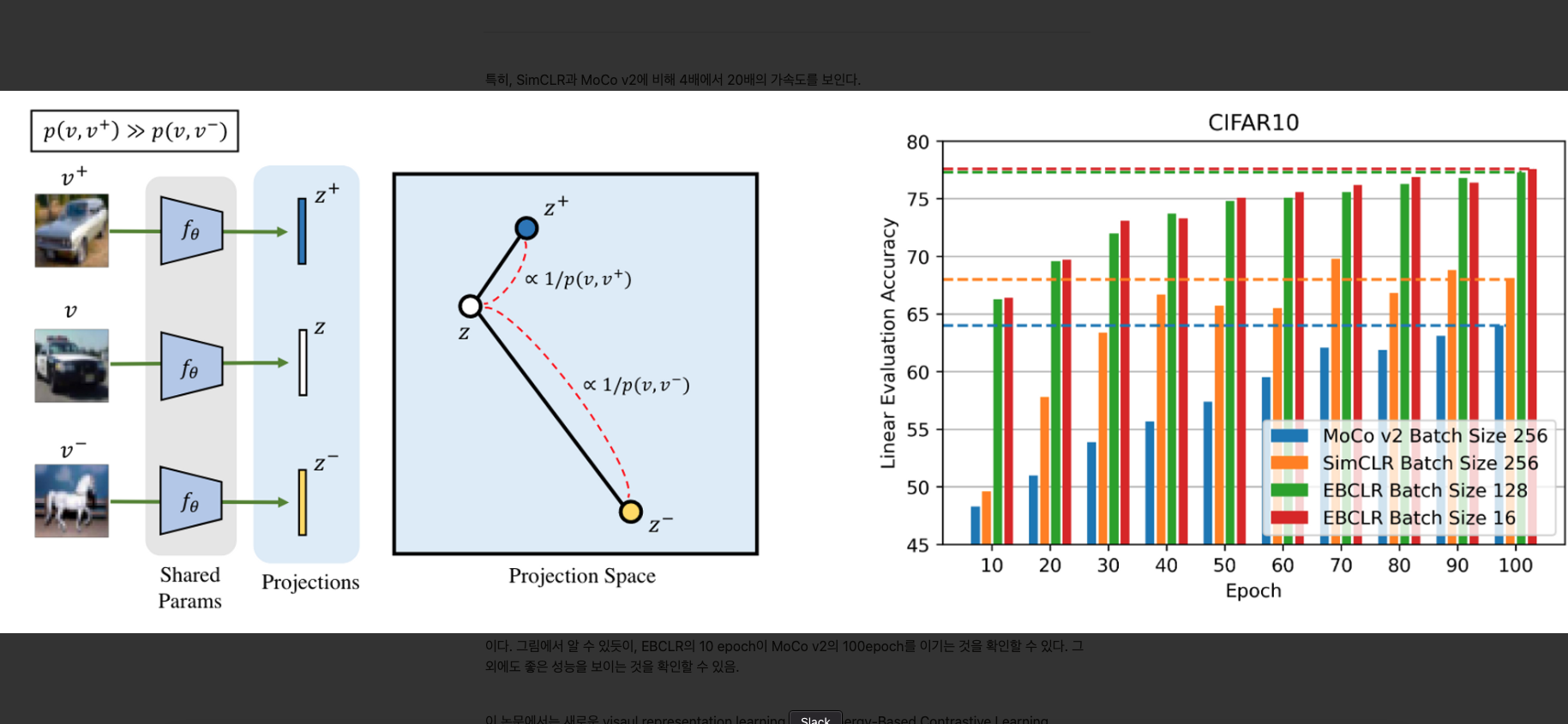
왼쪽 그림이 EBCLR을 잘 나타낸 그림이다. 여기서 $\propto$ 가 의미하는 것은 “is a monotonically increasing function of”이다. 여기서 논문의 저자들은 joint distribution $p(v,v^\prime)$를 사용하는데, 이것은 positive pairs의 joint distribution으로 이미지들의 semantic similarity를 측정한 것이다. 특별히, $p(v,v^\prime)$는 $v$와 $v^\prime$가 semantically similar할 때 높게 측정되고, 아닐때 낮게 측정된다. DNN $f_\theta$는 Projection space에서 보이는 거리로 훈련이 되는데, 이 거리가 $1/p(v,v^\prime)$ 으로부터 조절된다.

오른쪽 그림의 경우 EBCLR과 SimCLR, MoCo v2에서의 CIFAR10에 대한 linear evaluation accuracy 결과이다. 그림에서 알 수 있듯이, EBCLR의 10 epoch이 MoCo v2의 100epoch를 이기는 것을 확인할 수 있다. 그 외에도 좋은 성능을 보이는 것을 확인할 수 있음.

이 논문에서는 새로운 visaul representation learning 방법인 Energy-Based Contrastive Learning (EBCLR)방법을 제안한다. 이 방법은 leverages the power of geneartive learning by combining contrastive learning with energy-based models(EBMs).

EBCLR은 Contrastive learning loss를 generative loss로 보완하며, 이것은 positive pairs의 joint distribution 을 학습시키는 것으로 해석할 수 있다. 이를 통해, 기존의 Contrastive learning loss가 EBCLR의 특수한 경우임을 증명한다. 그리고 EBM은 SGLD에 의존하기 때문에, 훈련이 어려운 것으로 알려져 있지만, 논문에서는 특별한 SGLD를 제안하여 이를 극복하였다.

Related Works

EBCLR을 이해하기 위해서, EBM과 contrastive learning, generative model에 대해 간략하게 설명한다.

Contrastive Learning

한 배치의 이미지 $\{x_n\}^N_{n=1}$ 와 두개의 transformations $t,t^\prime$이 주어졌을 때, contrastive learning methods는 먼저 각 instance $x_n$에 대하여 이미지를 두개의 view로 만들어낸다. $v_n=t(x_n),v^\prime_n=t^\prime(x_n)$. 여기서 만약 $n=m$인 경우, pair $(v_n,v_m^\prime)$은 positive pair로 불리고 $n\neq m$인 경우는 negative pair로 불린다. DNN $f_\theta$가 주어질때, 이 view들은 $f_\theta$와 normalizing을 통해 projection space로 embedding된다.

Contrastive methods는 $f_\theta$가 positive pair의 projection에 대해서는 일치할 수 있도록 만들며, negative pairs에 대해서는 일치하지 않도록 학습한다. 특히, $f_\theta$는 InfoNCE objective를 최대화하기 위해 훈련된다. 훈련이 끝난 뒤에, $f_\theta$의 마지막 레이어 혹은 중간 레이어로부터 나오는 outputs들은 downstream task에 이용된다.

Energy-Based Models

scalar값을 가지는 energy function $E_\theta(v)$ with parameter $\theta$가 주어졌을 때, energy-based model(EBM)은 다음의 식으로부터 분포가 정의된다.

여기서 $Z(\theta)$는 partition function이며 $q_\theta$의 integrates가 1이 되도록 보장해준다. 여기에 필수적으로 energy function의 선택에 대한 아무런 제약이 존재하지 않기 때문에, EBM은 distributions을 모델링하는데 있어서 매우 유연하게 작동한다. 따라서 EBM은 매우 다양한 머신러닝 테스크(차원축소, generative classifier, generating images, 등등)에 사용된다. Wang은 EBM과 InfoNCE사이의 EBM의 generative performance를 향상시키는 연결에 대해 조사했는데, 이 논문에서는 처음으로 EBM을 representation learning을 위한 contrastive learning으로 사용하였다.

target distribution이 주어지면, EBM은 오직 $p$로부터 샘플링할 때, density $q_\theta$에 대해 추정할 수 있다. 이를 가능케하는 한가지 방법은 $q_\theta$와 $p$ 사이의 Kullback-Leibler (KL) divergence를 최소화하는 방법이며, $p$에 대하여, $q_\theta$의 log-likelihood의 기댓값을 최대화하는 것이다.

Stochastic gradient ascent가 이를 해결하기 위해 사용될 수 있다. 특히, paramether $\theta$의 관점에서 log-likelihood의 기댓값의 gradient는 다음과 같다.

유도

따라서, $\theta$를 업데이트 하는 것은 $q_\theta$로 부터 샘플링된 에너지에 대해 pulling up하는 것이고 $p$로부터 샘플링된 energy에 대해서는 pushing down하는 것이다. 이러한 optimization methods는 contrastive divergence로 잘 알려져있다.

위 식에서 두번째 있는 term $(-\mathbb{E}_p[\nabla_\theta E_\theta(v)])$는 $p$로부터 샘플함으로써 쉽게 계산될 수 있는 반면에, 첫번 째 텀은 $(\mathbb{E}_{q_\theta}[\nabla_\theta E_\theta(v)])$는 $q_\theta$로 부터 샘플이 필요하다. 이전 works들은 Stochastic Gradient Langevin Dynamic을 통해 $q_\theta$로 부터 샘플을 생성해준다. 특히, some proposal distribution $q_0$로부터의 하나의 샘플 $v_0$이 주어질때,

는 $\{v_t\}$의 시퀀스가 $q_\theta$로부터 나온 샘플로 converge함을 guarantee한다. (guarantees that the sequence $\{v_t\}$ converges to a sample from $q_\theta$ assuming $\{\alpha_t\}$ decays at a polynomial rate )

무슨 말이냐면, EBM은 위 생성된 샘플이 $q_\theta$에서 생성된 샘플이라는 것을 guarantee하는 방향으로 생성된다는 의미이다. 위의 에너지함수 $E_\theta(v_t)$의 $v_t$에 대한 미분값은 위 에너지 함수가 작아지는 방향으로 이미지를 만든다는 의미인데, 이 때 에너지함수가 작아진다는 것은 샘플 $v_t$가 분포 $q_\theta$에서 나올 확률을 높여준다는 것을 의미한다. 즉, step이 무한이 진행된다면 $\{v_t\}$의 시퀀스가 $q_\theta$로부터 나온 샘플임을 guarantee한다.

하지만, SGLD는 proposal distribution 로부터 나온 샘플이 target distribution로 converge할 때 까지 엄청나게 많은 step 수를 필요로 한다. 이것은 현실적으로 불가능하고, 오직 constant step size, i.e. $\alpha_t=\alpha$ 와 constant noise variance $\sigma_t=\sigma^2$ 가 사용된다. 게다가 Yang and Ji는 SGLD가 EBM을 훈련도중 발산하도록 하는 pixel값을 생성한다고 주장한다. 따라서 그들은 proximal SGLD라는 방법으로 gradient values를 threshold $\delta>0$을 갖는 특정 구간 $[-\delta,\delta]$로 clamp해줌으로써 EBM의 발산을 막는다. 따라서, update equation은

for $t=0,...T-1$, where $\epsilon\sim\mathcal{N}(0,\sigma^2)$ and clamp$\{\cdot,\delta\}$ clamps each element of the input vector into $[-\delta,\delta]$.

본 논문에서는 추가적인 수정을 통해 SGLD를 EBCLR에 더욱 가속해서 수렴하도록 만들었다.

Theory

Let $\mathcal{D}$ be a distribution of images and $\mathcal{T}$ a distribution of stochastic image transformations. Given $x\sim{\mathcal{D}}$ and i.i.d. $t,t^\prime\sim\mathcal{T}$, our goal is to approximate the joint distribution of the views

우선 $\mathcal{D}$라는 image distribution과 $\mathcal{T}$라는 image transformationdl 있다고 생각해보자. 주어진 분포 $\mathcal{D}$에서의 샘플 $x$,$x\sim\mathcal{D}$와 i.i.d $t,t^\prime\sim\mathcal{T}$, 에서 우리의 목표는 model distribution $q_\theta$를 사용해 실제 joint distribution $p$인 아래 분포를 잘 근사하는 것이다.

using the model distribution

where $Z(\theta)$ is a normalization constant, $\tau \gt0$ is a temperature hyper-parameter, and $z$ and $z^\prime$ are projections computed by passing the views $v$ and $v^\prime$ through the DNN $f_\theta$ and then normalizing to have unit norm. We now explain the intuitive meaning of matching $q_\theta$ to $p.$

본 논문의 키 아이디어는 $p(v,v^\prime)$을 $v$와 $v^\prime$의 semantic similarity를 측정하기 위해 사용한다는 것이다. 만약에 두 이미지 $v,v^\prime$이 semantically 비슷하다면, 그것들은 비슷한 이미지의 transformation일 가능성이 높다는 것을 의미할 것이다. 따라서 $p(v,v^\prime)$은 semantically 비슷한 $v,v^\prime$에서는 높고, 다른 경우에는 낮다.

$q_\theta$가 $p$를 아주 잘 근사한다고 가정하자. 만약 식 6번 처럼 식을 만들어 내고 $||z-z^\prime||$을 풀게 한다면, $z$와 $z^\prime$ 사이의 거리는 monotone increasing function of $1/p(v,v^\prime)$이 될 것이다. 이 $1/p(v,v^\prime)$은 $v,v^\prime$의 semantic similarity의 inverse이다. 따라서 semantically 비슷한 이미지들은 가까운 projections을 가지고, 다른 이미지들은 먼 projection을 가진다. 이것은 Figure.1을 보면 알 수 있다.

To approximate $p$ using $q_\theta$, we train $f_\theta$ to maximize the expected log-likelihood of $q_\theta$ under $p$:

In order to solve this problem with stochastic gradient ascent, we could naively extend (3) to the setting of joint distributions to obtain the following result.

Proposition 1

Proposition 1. The joint distribution (6) can be formulated as an EBM

and the gradient of the objective of (7) is given by

However, computing the first expectation in (9) requires sampling pairs of views $(v,v^\prime)$ from $q_\theta(v,v^\prime)$ via SGLD, which could be expensive. To avert this problem, we use Bayes’rule to decompose

모델에서 샘플링 된 데이터에 대한 에너지함수의 기댓값인 $\mathbb{E}_{q_\theta}[\nabla_\theta E_\theta(v,v^\prime)]$ 는 모델 $q_\theta$에서 샘플링 해야 된다는 치명적인 문제가 발생한다. 이러한 문제가 발생하지않게 하기 위해 베이즈룰을 이용해 위 식을 decompose해주면 아래와 같다.

위 식에서 우변의 첫번째와 두번째 term들은 각각 discriminative와 generative term을 나타낸다.

the first and second terms at the RHS will be referred to as discriminative and generative terms, respectively, throughout the paper. A similar decomposition was used by Grathwohl et al. in the setting of learning generative classifiers.

Furthermore, we add a hyper-parameter $\lambda$ to balance the strength of the disciriminative term and the generative term. The advantage of this modification will be discussed in Section 4.3. This yields our EBCLR objective

The discriminative term can be easily differentiated since the partition function $Z(\theta)$ cancels out when $q_\theta(v,v^\prime)$ is divided by $q_\theta(v)$. However, the generative term still contains $Z(\theta)$. We now present our key result, which is used to maximize (11). The proof is deferred to Appendix C.1.

What your classifier is hiding

최근 머신러닝에서, $K$ class를 갖는 분류 문제는 전형적으로 각각의 데이터 포인트 $\mathbf{x}\in\mathbb{R}^D$를 $K$ real-valued numbers known as logits로 맵핑해주는 parametric function, $f_\theta:\mathbb{R}^D\rightarrow\mathbb{R}^K$를 사용하여 푸는 것이다. 이러한 logits는 categorical distribution을 parameterize하는 것으로 사용되는데, 이 때 Softmax transfer function을 사용한다.

여기서 $f_\theta(\mathbf{x})[y]$ 는 $f_\theta(\mathbf{x})$의 $y^\text{th}$ index를 가리키고, logit은 $y^\text{th}$ class label을 의미한다.

논문의 저자의 주요한 관점은 다음과 같다.

$f_\theta$로 부터 얻은 logit을 $p(\mathbf{x},y)$와 $p(\mathbf{x})$로 약간 재해석할 수 있다는 것이다. $f_\theta$를 변화시키지 않고, logits을 재활용 하여 joint distribution of data point $\mathbf{x}$ and labels $y$ 에 기반한 energy based model을 만들어낼 수 있다 :

여기서 $Z(\theta)$는 unknown normalizing constant이고, $E_\theta(\mathbf{x},y)=-f_\theta(\mathbf{x})[y]$이다.

$y$를 marginalizing함으로써, unnormalized density model $\mathbf{x}$를 얻어낼 수 있다.

여기서 아무 분류기의 logtis의 $\text{LogSumExp}(\cdot)$은 $\mathbf{x}$ data point에서 energy function으로 정의되기 위해 재사용될 수 있다.

이게 무슨 말이냐면, 위에 $p_\theta(\mathbf{x})$에서의 Energy function $E_\theta(\mathbf{x})$가 energy based model 기준에서 $-\text{LogSumExp}$가 되어야 $p_\theta(\mathbf{x})$가 만들어진다는 의미이다.

---

---

where $Z(\theta)$ is the partition function in (6), and the gradient of the generative term is given by

Thus, the gradient of the EBCLR objective(14) is

Theorem 2 suggests that the EBM for the joint distribution can be learned by computing the gradients of the discriminative term and the EBM for the marginal distribution. Moreover, we only need to sample $v$ from $q_\theta(v)$ to compute the second expectation in (14).

Approximating the EBCLR Objective

To implement EBCLR, we need to approximate expectations in (11) with their empirical means.

For a given batch of images $\{x_n\}^N_{n=1}$ and two image transformations $t,t^\prime$, contrastive learning methods first create two views $v_n=t(x_n),v_n^\prime=t^\prime(x_n)$ of each instance $x_n$.

Suppose samples $\{(v_n,v^\prime_n)\}^N_{n=1}$ from $p(v,v^\prime)$ are given, and let $\{(z_n, z^\prime_n)\}^N_{n=1}$ be the corresponding projections. As the learning goal is to make $q_\theta(v_n, v^\prime_n)$ approximate the joint probability density function $p(v_n, v^\prime_n)$, the empirical mean $\hat{q_\theta}(v_n)$ can be defined as:

where the sum is over the collection of $v^\prime_m$ defined as

and $N^\prime :=|\{v^\prime_m:v^\prime_m\neq v_n\}|=2N-1$. One could also use a simpler form of the empirical mean :

Similarly, $q_\theta(v^\prime|v)$ in (11), which should approximate the conditional probability density $p(v^\prime|v)$, can be represented in terms of $q_\theta(v_n,v^\prime_n)$. Specifically, we have

It is then immediately apparent that the empirical form of the discriminative term using (18) is a particular instance of the contrastive learning objective such as InfoNCE and SimCLR. Hence, EBCLR can be interpreted as complementing contrastive learning with a generative term defined by an EBM.

For the second term, we use the simpler form of the empirical mean in (17):

We could also use (15) as the empirical mean, but either choice showed identical performance (see Appendix E.3.). So, we have found (15) to be not worth the additional complexity, and have resorted to the simpler approximation (17) instead. (17이 더 간단)

Modifications to SGLD

Theorem 2에 따르면, 식 14에서 두번째 기댓값을 계산하기 위해서는 marginal $q_\theta(v)$로부터의 샘플이 필요하다. 따라서, 이를 위해 proximal SGLD with the energy function (20)을 적용하면

$\text{for}\:t=0,...,T-1,\:\text{where}\:\epsilon\sim\mathcal{N}(0,\sigma^2)$이다. 본 논문에서는 proximal SGLD를 추가적으로 세가지를 수정한다. 지금부터 언급하는 SGLD는 아래의 proximal SGLD를 의미한다

첫번째로, 논문에서는 SGLD를 probability $\rho$를 가지고, 이전 iterations으로 부터 나온 generated samples 으로부터 initialize하고, 다시 SGLD chains를 proposal distribution $q_0$로부터 샘플링된 샘플로부터 reinitialize한다. 이것은 keeping a replay buffer $\mathcal{B}$ of SGLD samples from previous iterations를 통해 달성한다. 이러한 기술은 replay buffer를 유지하는 기술로, EBM의 convergence를 가속화시키고 안정화시키기 위해 중요한 기술이며, 이전 works에서 증명되었다.

First, we initialize SGLD from generated samples from previous iterations, and with probability $\rho$, we reinitialize SGLD chains from samples from a proposal distribution $q_0$. This is achieved by keeping a replay buffer $\mathcal{B}$ of SGLD samples from previous iterations. This technique of maintaining a replay buffer has also been used in previous works and has proven to be crucial for stabilizing and accelerating the convergence of EBMs.

Second, the proposal distribution $q_0$ is set to be the data distribution $p(v)$. This choice differs from those of previous works which have either used the uniform distribution or a mixture of Gaussians as the proposal distribution.

Finally, we use multi-stage SGLD (MSGLD), which adaptively controls the magnitude of noise added in SGLD. For each sample $\tilde{v}$ in the replay buffer $\mathcal{B}$, we keep a count $\kappa_{\tilde{v}}$ of number of times it has been used as the initial point of SGLD. For samples with a low count, we use noise of high variance, and for samples with a high count, we use noise of low variance. Specifically, in (5), we set

where $[\cdot]_+:=\max\{0,\cdot\},\sigma^2_{\max}\:\text{and}\:\sigma^2_{\min}$ are the upper and lower bounds on the noise variance, respectively, and $K$ controls the decay rate of noise variance. The purpose of this technique is to facilitate quick exploration of the modes of $q_\theta$ and still gurantee SGLD generates samples with sufficiently low energy. The pseudocodes for MSGLD and EBCLR are given in Algorithms 1 and 2, respectively, in Appendix B, and the overall learning flow of EBCLR is described in Figure 2.