[ICCV 2021]Energy-Based Open-World Uncertainty Modeling for Confidence Calibration (작성중)

ma-kjh·2023년 8월 29일

EBM

목록 보기

5/7

Abstract

Confidence calibration은 머신러닝 시스템의 의사 결정의 신뢰성에 있어서 중요하다. 그러나 deep neural network 기반의 discriminative classifier들은 종종 overconfident prediction으로 classification accuracy의 correctness likelihood를 반영하지 못하는 경우가 있다.

이러한 문제의 원인으로 본 논문은 the closed-world nature in softmax를 원인으로 주장한다. 왜냐하면 모델이 cross-entropy loss를 통해 훈련될 경우에, 이 모델의 input은 $K$ 개의 pre-defined된 category에서만 높은 확률을 가질 수 있기 때문이다.

이러한 문제를 해결하고자, 논문의 저자들은 새로운 $K+1$ -way softmax formulation을 제안한다. 이 방법은 추가적인 차원(extra dimension)으로써의 open-world uncertainty을 모델링하는 것을 포함하고 있다. 추가적 차원과 original $K$ -way 분류 문제를 학습시키는 것을 통합하기 위해, 새로운 energy-based objective function을 제안하고 나아가 이론적인 증명을 통한 objective가 extra dimension이 marginal data distribution을 포착할 수 있음을 증명한다.

이를 Energy-based Open-World Softmax (EOW-Softmax)라고 부르며, confidence calibration에서 sota를 달성했다.

Introduction

Method

A Brief Background on EBMs

EBM에서의 에너지함수 $E_\theta : \mathbb{R}^D\rightarrow\mathbb{R}$ (parametrized by $\theta$ ),는 $D$ -차원의 datapoint를 scalar로 mapping시키는 함수이다. 이 때, 학습은 $E_\theta$ 가 observed configurations of variables에 대해서는 low energy를 갖는다는 것이고, unobserved ones에 대해서는 high energy를 가져야 한다. $E_\theta$ 를 통해 any probability density $p(x)$ for $x\in\mathbb{R}^D$ 를 만들어 낼 수 있고 다음과 같다.

p_\theta(x)={\exp(-E_\theta(x))\over{Z(\theta)}}

여기서 $Z(\theta)=\int_x\exp(-E_\theta(x))$ 로, normalizing constant를 나타내며 partition function으로 알려져있다. 우리는 여기서의 $E_\theta$ 를 deep neural network로 표현할 것이다. 일반적으로 EBM을 optimize할 때, Markov Chain Monte Carlo (MCMC)와 같은 샘플링 방법을 통해 모델로부터의 샘플을 필요로한다.

Energy-Based Open-World Softmax

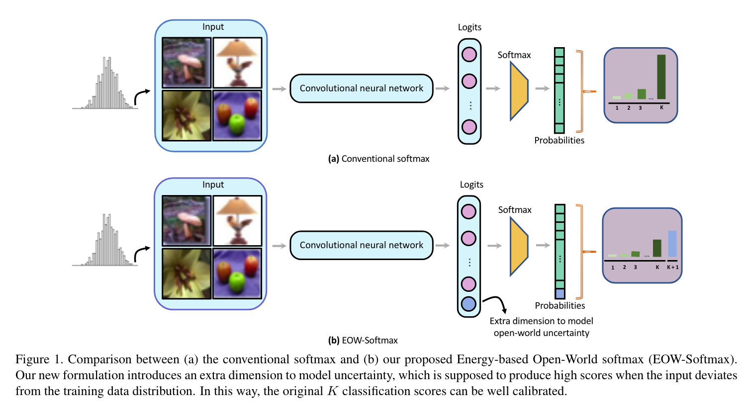
Open-World Softmax

이전에도 언급했듯이, 일반적인 softmax-based classifier같은 경우 open-world uncertainty를 모델링하는 능력이 떨어진다. 이를 해결하기 위해, output probability에 대해 $K+1$ 개의 카테고리를 사용하여 $K+1$ 번째 score가 open-world uncertainty를 나타낼 수 있도록 해준다. 이 때, 네트워크는 abnormal input에 대해서는 high uncertainty score를 생성하도록 만들어주는데, 이는 original $K$ category에 대한 예측의 confidence를 낮출 수 있을 것이다.

$f_\theta:\mathbb{R}^D\rightarrow\mathbb{R}^{K+1}$ 를 우리가 가진 $K+1$ 번째 logits을 생성하는 neural network model (excluding the softmax layer)라고 가정하고, $f_\theta(x)[i]$ 를 $x$ 가 주어졌을 때, %i%번 째, $i\in\{1,...,K,K+1\}$ , logit에 대한 예측값이라고 해보자. 출력 확률은 다음과 같이 얻어진다.

h_\theta(x)[i]={\exp(f_\theta(x)[i])\over{\sum^{K+1}_{j=1}\exp (f_\theta(x)[j])}}

여기서 $h_\theta$ 는 combination of the neural network $f_\theta$ 이다.

Energy-Based Learning Objective

그럼 여기서, $h_\theta(x)[K+1]$ 을 uncertainty로 encode할 수 있게 어떻게 learning objective를 설정할 수 있을까? 논문의 아이디어는 해당 $h_\theta(x)[K+1]$ 를 marginal data distribution의 score로 연관지었다.

직관적으로 입력이 훈련 데이터 분포 $p(x)$ 에서 온다고 했을 때, 모델은 결정에 자신감을 가지게 될 것이다. 그렇다면 $h_\theta(x)[K+1]$ 는 낮아져야 할 것이다(conversely, $\sum^K_{i=1}h_\theta(x)[i]$ should be high). 만약에 입력이 training data distribution에 다르다면, 모델은 결정에 불확실할 것이고, 이 경우에는 $h_\theta(x)[K+1]$ 은 높은 수준의 uncertainty를 가지고 있어야 하며, 이는 자연스럽게 $\sum^K_{i=1}h_\theta(x)[i]$ 는 낮게 형성될 것이다 (due to the softmax normalization). 하지만, 직접적으로 $h_\theta(x)[K+1]$ 를 marginal distribution $p(x)$ (i.e. generative modeling)를 capture하는 것은 어렵다. 대신에, 논문에서는 EBMs의 도움을 받아 문제를 해결하고자 한다.

먼저 에너지함수를 정의한다.

E_\theta(x) = \log h_\theta(x)[K+1].

그리고 나서, objective를 정의하면 다음과 같다.

\min_\theta \mathbb{E}_{p(x)}[-\log h_\theta(x)[y]]+\lambda\mathbb{E}_{p_{\bar{\theta}}(x)} [-\log h_\theta(x)[K+1]],

이며 이 때 $\lambda$ 는 하이퍼파라미터이다.

이 때, 첫번째 텀은 K-way classification task의 ground-truth label $y$ 에 대한 maximum log-likelihood objective를 의미하고, 두번 째 텀은 $p_{\bar{\theta}}(x)$ 로 부터 샘플링된 데이터에 대한 maximum log-likelihood objective 이다.

$p_{\bar{\theta}(x)}$ 는 model distribution을 의미하며 특정 iteration의 frozen parameters of $p_\theta(x)$ 의 model distribution이다.

위 식은 original class들의 나머지 $K$ softmax score의 합을 이용해 marginal density $p(x)$ 를 직접적으로 구하고, 이는 $K+1$ 번 째 softmax score의 negatively correlated to $p(x)$ 로 만들어줄 것이다.

SGLD-Based Optimization

objective의 second term을 optimization하기 위해, sampler기반의 방법이 존재하고, 일반적으로 MCMC기반의 Stochastic Gradient Langevin Dynamics (SGLD)를 이용한다. SGLD sampling process는 아래와 같다.

z_{t+1} = z_t - {\alpha\over{2}}{\partial E_\theta(z_t)\over{\partial z_t}}+\sqrt{\epsilon},\:\:\epsilon\sim\mathcal{N}(0,I),

이 때 $t$ 는 SGLD의 iteration을 의미하며, $\alpha$ 는 스텝사이즈, 그리고 $\epsilon$ 은 정규분포로 부터 추출된 랜덤 노이즈이다. 실제로 $\alpha$ 는 일반적으로 고정한다.

대부분의 SGLD-based 방법들은 샘플을 이미지 공간에서 추출하게 된다. 이것은 정보가 전체 neural network를 통해서 흐르기 때문에 굉장히 계산적으로 비용이 높다. 따라서 논문에서는 latent space에서 샘플을 뽑는 것으로 문제를 해결하고자 했다. 따라서 위 식의 $z$ 는 image가 아닌 feature를 의미한다. 이러한 디자인은 훈련을 빠르게 만들 뿐 아니라, 정보가 network model의 일부만을 거치기 때문에 훨씬 깊은 아키텍쳐에서 한정된 자원으로도 학습이 가능하다. 게다가 이러한 latent space는 일반적으로 image space보다 smoother한 것이 알려져 있고, gradient를 계산하는데 용이하다.

Theoretical Insight

본 논문의 objective가 $h_\theta(x)[K+1]$ negatively correlated with $p(x)$ 하다는 것을 증명하기 위해, EBM modeled distribution인 $q_\theta(x)$ 를 $p(x)$ 에 KL divergence를 이용하여 minimize하는 것으로 기존 objective를 해석한다.