https://arxiv.org/abs/2203.13455
Contrastive Energy-based Models (CEM)
Adversarial Training (AT)는 딥러닝 네트워크의 robustness를 향상시켜주는 효과적인 방법 으로 잘 알려져 있다. 최근 많은 연구자들이 이러한 AT로 훈련된 robust한 모델이 좋은 생성 능력을 가지고 진짜같은 이미지를 생성할 수 있다는 사실을 알았지만, 아직까지 왜 이것이 잘 되는지에 대한 이유는 미지수 였다.
이 논문은 이러한 현상을 Contrastive Energy-based Models(CEM) 이라는 통합된 확률적 프레임워크로 해석했다. 한편으로 첫번째로 이러한 통합된 robustness와 생성 능력의 이해 를 통해 AT의 probabilistic characterization을 제공한다. 또 한편으로는, 이 논문에서 제안하는 통합된 프레임워크가 unsupervised scenario로 확장됨으로써, unsupervised contrastive learning을 important sampling of CEM으로 해석 할 수 있음을 보여준다.
이를 기반으로, 논문의 저자들은 adversarial learning과 sampling method를 발전시킬 수 있는 principled method에 대해 제안한다.
한 줄로 요약하면 다음과 같다.
Energy Based modeling을 통해 adversarial training이 왜 잘 작동되는지 해석해보자.
Adversarial Training (AT)는 딥러닝 네트워크의 robustness를 향상시킬 수 있는 가장 효과적인 방법중 하나 로 지금까지 발전되어 왔다. AT는 minimax optimization problem을 푸는데, adversarial example을 classification loss를 최대화 함으로써 생성하는 inner maximization 과 maximization으로 만들어진 adversarial example의 classification loss를 최소화 하는 model의 parameter를 찾는 outer minimization 두가지의 minimax optimization이다.
최근들어, 연구자들에 의해 AT를 통해 얻어진 robust classifier가 perceptually aligned with human방식으로 features를 추출할 수 있도록 한다고 알려져 있다. 그럼에도, 이러한 AT가 왜 더 의미적으로 의미있는 특징을 뽑고 classifier를 generator로 학습할 수 있는지에 대한 이유는 알지 못해왔다.
게다가 AT의 경우 훈련시에 deep generative model가 { x i } \{\mathbf{x}_i\} { x i } { ( x i , y i ) } \{(\mathbf{x}_i,\mathbf{y}_i)\} { ( x i , y i ) }
그럼 이제 왜 잘되는지 파해쳐보자.
CEM : A Unified Probabilistic Framework
이전의 연구중에 discriminative model을 energy-based model로 연결하는 연구들이 있었는데, 이 연구에서 저자는 Contrastive Energy-based Model(CEM)을 제안함으로써 supervised와 unsupervised scenarios를 통합한다.
저자의 제안된 CEM은 특정 Energy-based Model (EBM)이며, joint distribution p θ ( u , v ) p_\theta(\mathbf{u,v}) p θ ( u , v ) ( u , v ) \mathbf{(u,v)} ( u , v ) f θ ( u , v ) f_\theta(\mathbf{u,v}) f θ ( u , v )
p θ ( u , v ) = exp ( f θ ( u , v ) ) Z ( θ ) p_\theta(\mathbf{u,v})={\exp(f_\theta(\mathbf{u,v}))\over{Z(\theta)}} p θ ( u , v ) = Z ( θ ) exp ( f θ ( u , v ) ) 여기서 Z ( θ ) = ∫ exp ( f θ ( u , v ) ) d u d v Z(\theta)=\int\exp(f_\theta(\mathbf{u,v}))d\mathbf{u}d\mathbf{v} Z ( θ ) = ∫ exp ( f θ ( u , v ) ) d u d v ( u , v ) (\mathbf{u,v}) ( u , v )
Parametric CEM
supervised scenario에서, 논문의 저자는 Parametric CEM (P-CEM)이라는 것으로 joint distribution p θ ( x , y ) p_\theta(\mathbf{x},y) p θ ( x , y ) x \mathbf{x} x y y y
p θ ( x , y ) = exp ( f θ ( x , y ) ) Z ( θ ) = exp ( g θ ( x ) ⊤ w y ) Z ( θ ) p_\theta(\mathbf{x},y)={\exp(f_\theta(\mathbf{x},y))\over{Z(\theta)}}={\exp(g_\theta(\mathbf{x})^\top \mathbf{w}_y)\over{Z(\theta)}} p θ ( x , y ) = Z ( θ ) exp ( f θ ( x , y ) ) = Z ( θ ) exp ( g θ ( x ) ⊤ w y ) 여기서 g θ : R n → R m g_\theta:\mathbb{R}^n\rightarrow \mathbb{R}^m g θ : R n → R m g ( x ) ∈ R m g(\mathbf{x})\in\mathbb{R}^m g ( x ) ∈ R m x \mathbf{x} x w k ∈ R m \mathbf{w}_k\in\mathbb{R}^m w k ∈ R m k k k
linear classification weight인 W = [ w 1 , ⋯ , w K ] \mathbf{W}=[\mathbf{w}_1,\cdots,\mathbf{w}_K] W = [ w 1 , ⋯ , w K ] h ( x ) = g ( x ) ⊤ W h(\mathbf{x})=g(\mathbf{x})^\top\mathbf{W} h ( x ) = g ( x ) ⊤ W
f θ ( x , y ) = g θ ( x ) ⊤ w y = h θ ( x ) [ y ] f_\theta(\mathbf{x},y)=g_\theta(\mathbf{x})^\top\mathbf{w}_y=h_\theta(\mathbf{x})[y] f θ ( x , y ) = g θ ( x ) ⊤ w y = h θ ( x ) [ y ] Non-Parametric CEM
Unsupervised scenario에서, 논문의 저자는 label에 access하지 않고 joint distribution을 ( x , x ′ ) (\mathbf{x},\mathbf{x}^\prime) ( x , x ′ )
p θ ( x , x ′ ) = exp ( f θ ( x , x ′ ) ) Z ( θ ) = exp ( g θ ( x ) ⊤ g θ ( x ′ ) ) Z ( θ ) p_\theta(\mathbf{x},\mathbf{x}^\prime)={\exp(f_\theta(\mathbf{x},\mathbf{x}^\prime))\over{Z(\theta)}}={\exp(g_\theta(\mathbf{x})^\top g_\theta(\mathbf{x}^\prime))\over{Z(\theta)}} p θ ( x , x ′ ) = Z ( θ ) exp ( f θ ( x , x ′ ) ) = Z ( θ ) exp ( g θ ( x ) ⊤ g θ ( x ′ ) ) 그러고 나면 이러한 Non-parametric CEM의 likelihood gradient과 상응되는 것은 다음과 같다.이 논문을 먼저 보면 조금 이해가 편해짐
∇ θ E p d ( x , x ′ ) log p θ ( x , x ′ ) = E p d ( x , x ′ ) ∇ θ f θ ( x , x ′ ) − E p θ ( x ^ , x ^ ′ ) ∇ θ f θ ( x ^ , x ^ ′ ) \nabla_\theta\mathbb{E}_{p_d(\mathbf{x},\mathbf{x}^\prime)}\log p_\theta(\mathbf{x},\mathbf{x}^\prime)=\mathbb{E}_{p_d(\mathbf{x},\mathbf{x}^\prime)}\nabla_\theta f_\theta(\mathbf{x},\mathbf{x}^\prime) -\mathbb{E}_{p_\theta(\hat{\mathbf{x}},\hat{\mathbf{x}}^\prime)}\nabla_\theta f_\theta(\hat{\mathbf{x}},\hat{\mathbf{x}}^\prime) ∇ θ E p d ( x , x ′ ) log p θ ( x , x ′ ) = E p d ( x , x ′ ) ∇ θ f θ ( x , x ′ ) − E p θ ( x ^ , x ^ ′ ) ∇ θ f θ ( x ^ , x ^ ′ ) P-CEM이 parametric cluster center를 포함(데이터 x x x y y y ( x , x ′ ) (\mathbf{x},\mathbf{x}^\prime) ( x , x ′ ) p d ( x , x ′ ) = p d ( x ) p d ( x ′ ∣ x ) p_d(\mathbf{x},\mathbf{x}^\prime)=p_d(\mathbf{x})p_d(\mathbf{x}^\prime|\mathbf{x}) p d ( x , x ′ ) = p d ( x ) p d ( x ′ ∣ x )
x ′ = f θ ( t ( x ) ) , t ∼ u . a . r . T , x ∼ p d ( x ) \mathbf{x}^\prime=f_\theta(t(\mathbf{x})),\:\:\:\:\:t\mathop{\sim}\limits^{u.a.r.}\mathcal{T},\:\:\:\mathbf{x}\sim p_d(\mathbf{x}) x ′ = f θ ( t ( x ) ) , t ∼ u . a . r . T , x ∼ p d ( x ) u . a . r u.a.r u . a . r
T = { t : R n → R n } \mathcal{T}=\{t:\mathbb{R}^n\rightarrow\mathbb{R}^n\} T = { t : R n → R n }
논문에서는 empirical data distribution p d ( x ) p_d(\mathbf{x}) p d ( x ) X \mathcal{X} X
Adversarial Training
Adversarial Training의 objective는 다음과 같다.
min θ E p d ( x , y ) [ max ∣ ∣ x ^ − x ∣ ∣ p ≤ ϵ ℓ CE ( x ^ , y ; θ ) ] , where ℓ CE = − log p θ ( y ∣ x ^ ) ( 7 ) \min_\theta\mathbb{E}_{p_d(\mathbf{x},y)}[\max_{||\hat{\mathbf{x}}-\mathbf{x}||_p\leq \epsilon}\ell_{\text{CE}}(\hat{\mathbf{x}},y;\theta)],\:\:\:\text{where}\:\:\ell_\text{CE}=-\log p_\theta(y|\hat{\mathbf{x}})\:\:\: (7) θ min E p d ( x , y ) [ ∣ ∣ x ^ − x ∣ ∣ p ≤ ϵ max ℓ CE ( x ^ , y ; θ ) ] , where ℓ CE = − log p θ ( y ∣ x ^ ) ( 7 ) 식에서 볼 수 있듯이, p d ( x , y ) p_d(\mathbf{x},y) p d ( x , y ) ( x , y ) (\mathbf{x},y) ( x , y ) ℓ CE \ell_\text{CE} ℓ CE θ \theta θ x ^ \hat{\mathbf{x}} x ^ ℓ CE \ell_\text{CE} ℓ CE
Maximization Process
inner maximization problem에서, Projected Gradient Descent (PGD) 는 CE loss를 maximizing함 으로써 adversarial example x ^ \hat{\mathbf{x}} x ^ 하는 일반적인 방법이다. (i.e., minimizing the log conditional probability) starting from x ^ 0 = x : \hat{\mathbf{x}}_0=\mathbf{x}: x ^ 0 = x :
Projected Gradient Descent (PGD)
x ^ n + 1 = x ^ n + α ∇ x ^ n ℓ ( x ^ n , y ; θ ) = x ^ n − α ∇ x ^ n log p θ ( y ∣ x ^ n ) = x ^ n + α ∇ x ^ n [ log ∑ k = 1 K exp ( f θ ( x ^ n , k ) ) ] − α ∇ x ^ n f θ ( x ^ n , y ) , \hat{\mathbf{x}}_{n+1}=\hat{\mathbf{x}}_n+\alpha\nabla_{\hat{\mathbf{x}}_n}\ell(\hat{\mathbf{x}}_n,y;\theta)=\hat{\mathbf{x}}_n-\alpha\nabla_{\hat{\mathbf{x}}_n}\log p_\theta(y|\hat{\mathbf{x}}_n)\\ =\hat{\mathbf{x}}_n+\alpha\nabla_{\hat{\mathbf{x}}_n}[\log\sum^K_{k=1}\exp(f_\theta(\hat{\mathbf{x}}_n,k))] -\alpha\nabla_{\hat{\mathbf{x}}_n}f_\theta(\hat{\mathbf{x}}_n,y), x ^ n + 1 = x ^ n + α ∇ x ^ n ℓ ( x ^ n , y ; θ ) = x ^ n − α ∇ x ^ n log p θ ( y ∣ x ^ n ) = x ^ n + α ∇ x ^ n [ log k = 1 ∑ K exp ( f θ ( x ^ n , k ) ) ] − α ∇ x ^ n f θ ( x ^ n , y ) , 반면에, Langevin dynamics for sampling P-CEM은, random noise x ^ 0 = δ \hat{\mathbf{x}}_0=\delta x ^ 0 = δ
Stochastic Gradient Langevin dynamics (SGLD)
x ^ n + 1 = x ^ n + α ∇ x ^ log p θ ( x ^ n ) + 2 α ⋅ ϵ = x ^ n + α ∇ x ^ n [ log ∑ k = 1 K exp ( f θ ( x ^ n , k ) ) ] + 2 α ⋅ ϵ . \hat{\mathbf{x}}_{n+1}=\hat{\mathbf{x}}_n+\alpha\nabla_{\hat{\mathbf{x}}}\log p_\theta(\hat{\mathbf{x}}_n)+\sqrt{2\alpha} \cdot \epsilon\\=\hat{\mathbf{x}}_n+\alpha\nabla_{\hat{\mathbf{x}}_n}[\log\sum^K_{k=1}\exp(f_\theta(\hat{\mathbf{x}}_n,k))]+\sqrt{2\alpha}\cdot\epsilon. x ^ n + 1 = x ^ n + α ∇ x ^ log p θ ( x ^ n ) + 2 α ⋅ ϵ = x ^ n + α ∇ x ^ n [ log k = 1 ∑ K exp ( f θ ( x ^ n , k ) ) ] + 2 α ⋅ ϵ . 위 두 Equation 모두 positive logsumexp gradient 을 가지며(이는 EBM관점에서 E ( x ^ ) E(\hat{\mathbf{x}}) E ( x ^ ) marginal probability p θ ( x ^ ) p_\theta(\hat{\mathbf{x}}) p θ ( x ^ ) 이다. PGD의 세번째 텀은 original data point로 부터 멀리 떨어진 repulsive gradient를 필요로 하면서 local region을 exploration하는 data point ( x , y ) (\mathbf{x},y) ( x , y ) ϵ \epsilon ϵ
JEM에서 보았던 것과의 차이는 아래와 같다.
Comparing PGD and Langevin
위 두 분석을 통해, maximization process in AT 는 probabilistic model p θ ( x ^ ) p_\theta(\hat{\mathbf{x}}) p θ ( x ^ ) biased sampling method의 하나 로 바라볼 수 있다. Langevin dynamics와 비교했을 때, PGD의 경우 sampling에서 inductive bias를 강요 한다.
추가적인 repulsive gradient 그리고 ϵ \epsilon ϵ 샘플이 오리지널 데이터 포인트 근처에서 misclassified되는 샘플을 뽑도록 만들어준다 .(− α ∇ x ^ n f θ ( x ^ n , y ) -\alpha\nabla_{\hat{\mathbf{x}}_n}f_\theta(\hat{\mathbf{x}}_n,y) − α ∇ x ^ n f θ ( x ^ n , y ) 더 stable하며 , 이것은 PGD attack이 JEM training을 통한 negative sampling 방법을 대체 할 수 있는 경쟁력있는 하나의 수단임을 암시한다.
Minimization process
P-CEM을 위한 joint log likelihood의 gradient를 시작
∇ θ E p d ( x , y ) log p θ ( x , y ) = E p d ( x , y ) ∇ θ f θ ( x , y ) − E p θ ( x ^ , y ^ ) ∇ θ f θ ( x ^ , y ^ ) = E p d ( x , y ) ∇ θ f θ ( x , y ) − E p θ ( x ^ ) p θ ( y ^ ∣ x ^ ) ∇ θ f θ ( x ^ , y ^ ) , \nabla_\theta \mathbb{E}_{p_d(\mathbf{x},y)}\log p_\theta(\mathbf{x},y)\\=\mathbb{E}_{p_d(\mathbf{x},y)}\nabla_\theta f_\theta(\mathbf{x},y)-\mathbb{E_{p_\theta(\hat{\mathbf{x}},\hat{y})}}\nabla_\theta f_\theta(\hat{\mathbf{x}},\hat{y})\\ =\mathbb{E}_{p_d(\mathbf{x},y)}\nabla_\theta f_\theta(\mathbf{x},y)-\mathbb{E}_{p_\theta(\hat{\mathbf{x}})p_\theta(\hat{y}|\hat{\mathbf{x}})}\nabla_\theta f_\theta(\hat{\mathbf{x}},\hat{y}), ∇ θ E p d ( x , y ) log p θ ( x , y ) = E p d ( x , y ) ∇ θ f θ ( x , y ) − E p θ ( x ^ , y ^ ) ∇ θ f θ ( x ^ , y ^ ) = E p d ( x , y ) ∇ θ f θ ( x , y ) − E p θ ( x ^ ) p θ ( y ^ ∣ x ^ ) ∇ θ f θ ( x ^ , y ^ ) , ( x , y ) ∼ p d ( x , y ) (\mathbf{x},y)\sim p_d(\mathbf{x},y) ( x , y ) ∼ p d ( x , y )
( x ^ , y ^ ) ∼ p θ ( x ^ , y ^ ) (\hat{\mathbf{x}},\hat{y})\sim p_\theta(\hat{\mathbf{x}},\hat{y}) ( x ^ , y ^ ) ∼ p θ ( x ^ , y ^ ) x ^ \hat{\mathbf{x}} x ^ y ^ ∼ p θ ( y ^ ∣ x ^ ) \hat{y}\sim p_\theta(\hat{y}|\hat{\mathbf{x}}) y ^ ∼ p θ ( y ^ ∣ x ^ ) x ^ \hat{\mathbf{x}} x ^
Minimization process에서는 P-CEM의 likelihood를 maximum하는 것이 AT의 minimization과 어떤 관련이 있는지 볼 것 이다.
논문에서는 interpolated adversarial pair ( x ^ , y ) (\hat{\mathbf{x}},y) ( x ^ , y )
∇ θ E p d ( x , y ) log p θ ( x , y ) = E p d ( x , y ) ⊗ p θ ( x ^ , y ^ ) [ ∇ θ f θ ( x , y ) − ∇ θ f θ ( x ^ , y ^ ) ] = E p d ( x , y ) ⊗ p θ ( x ^ , y ^ ) [ ∇ θ f θ ( x , y ) − ∇ θ f θ ( x ^ , y ) + ∇ θ f θ ( x ^ , y ) − ∇ θ f θ ( x ^ , y ^ ) . ] \nabla_\theta\mathbb{E}_{p_d(\mathbf{x},y)}\log p_\theta(\mathbf{x},y)=\mathbb{E}_{p_d(\mathbf{x},y)\otimes p_\theta(\hat{\mathbf{x}},\hat{y})}[\nabla_\theta f_\theta(\mathbf{x},y)-\nabla_\theta f_\theta(\hat{\mathbf{x}},\hat{y})]\\=\mathbb{E_{p_d(\mathbf{x},y)\otimes p_\theta(\hat{\mathbf{x}},\hat{y})}}[\nabla_\theta f_\theta(\mathbf{x},y)-\nabla_\theta f_\theta(\hat{\mathbf{x}},y)+\nabla_\theta f_\theta(\hat{\mathbf{x}},y)-\nabla_\theta f_\theta(\hat{\mathbf{x}},\hat{y}).] ∇ θ E p d ( x , y ) log p θ ( x , y ) = E p d ( x , y ) ⊗ p θ ( x ^ , y ^ ) [ ∇ θ f θ ( x , y ) − ∇ θ f θ ( x ^ , y ^ ) ] = E p d ( x , y ) ⊗ p θ ( x ^ , y ^ ) [ ∇ θ f θ ( x , y ) − ∇ θ f θ ( x ^ , y ) + ∇ θ f θ ( x ^ , y ) − ∇ θ f θ ( x ^ , y ^ ) . ] 앞에 있는 텀이 consistency gradient, 뒤에 텀이 contrastive gradient.
그리고 나서, 이 두 파트가 두가지 효과적인 메커니즘을 adversarial training에서 상응한다는걸 보여준다.
AT loss
contrastive gradient(뒤에 텀)에서 두가지 샘플 페어는 같은 입력인 x ^ \hat{\mathbf{x}} x ^
min θ E p d ( x , y ) [ max ∣ ∣ x ^ − x ∣ ∣ p ≤ ϵ ℓ CE ( x ^ , y ; θ ) ] , where ℓ CE = − log p θ ( y ∣ x ^ ) ( 7 ) \min_\theta\mathbb{E}_{p_d(\mathbf{x},y)}[\max_{||\hat{\mathbf{x}}-\mathbf{x}||_p\leq \epsilon}\ell_{\text{CE}}(\hat{\mathbf{x}},y;\theta)],\:\:\:\text{where}\:\:\ell_\text{CE}=-\log p_\theta(y|\hat{\mathbf{x}})\:\:\: (7) θ min E p d ( x , y ) [ ∣ ∣ x ^ − x ∣ ∣ p ≤ ϵ max ℓ CE ( x ^ , y ; θ ) ] , where ℓ CE = − log p θ ( y ∣ x ^ ) ( 7 ) E p d ( x , y ) ⊗ p θ ( x ^ , y ^ ) [ ∇ θ f θ ( x ^ , y ) − ∇ θ f θ ( x ^ , y ^ ) ] = E p d ( x , y ) ⊗ p θ ( x ^ ) [ ∇ θ f θ ( x ^ , y ) − E p θ ( y ^ ∣ x ^ ) ∇ θ f θ ( x ^ , y ^ ) ] = E p d ( x , y ) ⊗ p θ ( x ^ ) ∇ θ log p θ ( y ∣ x ^ ) \mathbb{E}_{p_d(\mathbf{x},y)\otimes p_\theta(\hat{\mathbf{x}},\hat{y})}[\nabla_\theta f_\theta(\hat{\mathbf{x}},y)-\nabla_\theta f_\theta(\hat{\mathbf{x}},\hat{y})]\\=\mathbb{E}_{p_d(\mathbf{x},y)\otimes p_\theta(\hat{\mathbf{x}})}[\nabla_\theta f_\theta(\hat{\mathbf{x}},y)-\mathbb{E}_{p_\theta(\hat{y}|\hat{\mathbf{x}})}\nabla_\theta f_\theta(\hat{\mathbf{x}},\hat{y})]\\=\mathbb{E}_{p_d(\mathbf{x},y)\otimes p_\theta(\hat{\mathbf{x}})}\nabla_\theta \log p_\theta(y|\hat{\mathbf{x}}) E p d ( x , y ) ⊗ p θ ( x ^ , y ^ ) [ ∇ θ f θ ( x ^ , y ) − ∇ θ f θ ( x ^ , y ^ ) ] = E p d ( x , y ) ⊗ p θ ( x ^ ) [ ∇ θ f θ ( x ^ , y ) − E p θ ( y ^ ∣ x ^ ) ∇ θ f θ ( x ^ , y ^ ) ] = E p d ( x , y ) ⊗ p θ ( x ^ ) ∇ θ log p θ ( y ∣ x ^ ) 이는 정확하게 negative gradient robust CE loss (AT loss) in EQ 7와 동일하다. 다른말로, gradient ascent with the contrastive gradient is equivalent to gradient descent w.r.t. the AT loss .
즉, log p θ ( y ∣ x ^ ) \log p_\theta(y|\hat{\mathbf{x}}) log p θ ( y ∣ x ^ ) − log p θ ( y ∣ x ^ ) -\log p_\theta(y|\hat{\mathbf{x}}) − log p θ ( y ∣ x ^ )
Regularization. (?)
consistency gradient에서, original AT는 간단하게 무시된다. 변화된 버전인 TRADES는 대신에 KL regularization인 KL ( p ( ⋅ ∣ x ^ ) ∣ ∣ p ( ⋅ ∣ x ) ) \text{KL}(p(\cdot|\hat{\mathbf{x}})||p(\cdot|\mathbf{x})) KL ( p ( ⋅ ∣ x ^ ) ∣ ∣ p ( ⋅ ∣ x ) ) p ( ⋅ ∣ x ^ ) = p ( ⋅ ∣ x ) → f θ ( x , y ) = f θ ( x ^ , y ) p(\cdot|\hat{\mathbf{x}})=p(\cdot|\mathbf{x})\rightarrow f_\theta(\mathbf{x},y)=f_\theta(\hat{\mathbf{x}},y) p ( ⋅ ∣ x ^ ) = p ( ⋅ ∣ x ) → f θ ( x , y ) = f θ ( x ^ , y )
Comparing AT and JEM training paradigms.
위 분석을 토대로, AT의 minimization objective는 JEM의 maximum likelihood training과 관련이 되어있다.
joint likelihood를 p θ ( x ) p_\theta(\mathbf{x}) p θ ( x ) p θ ( y ∣ x ) p_\theta(y|\mathbf{x}) p θ ( y ∣ x ) ( x , y ) (\mathbf{x},y) ( x , y ) ( x ^ , y ^ ) (\hat{\mathbf{x}},\hat{y}) ( x ^ , y ^ ) ( x ^ , y ) (\hat{\mathbf{x}},y) ( x ^ , y )
게다가 이것은 consistency gradient를 regularization함으로써 adversarial robustness bias를 주입할 수 있게된다. 이와 함께 maximization process에서의 논문의 분석에서, AT가 더 안정적인 JEM training을 위한 경쟁적인 대안이 될 수 있다. 이는 AT로 훈련된 robust model이 왜 generative 한지에 대해서도 설명된다.
Proposed Supervised Adversarial sampling algoritms
본 논문의 해석은 또한 robust classifier를 위한 sampling algorithm의 중요한 디자인에 영감을 줄 수 있다.
Targeted Attack (TA)
이전의 robust classifier의 경우 sample을 추출하기 위해서, JEM같은 경우 targeted attack을 이용했다. 이 targeted attack은 random initialized input x ^ 0 \hat{\mathbf{x}}_0 x ^ 0 y ^ \hat{y} y ^
x ^ n + 1 = x ^ n + α ∇ x n log p θ ( y ^ ∣ x ^ n ) = x ^ n + α ∇ x f ( x ^ n , y ^ ) − α ∇ x ^ n [ log ∑ k = 1 K exp ( f θ ( x ^ n , k ) ) ] . \hat{\mathbf{x}}_{n+1}=\hat{\mathbf{x}}_n+\alpha \nabla_{\mathbf{x}_n}\log p_\theta(\hat{y}|\hat{\mathbf{x}}_n)=\hat{\mathbf{x}}_n+\alpha\nabla_\mathbf{x}f(\hat{\mathbf{x}}_n,\hat{y})-\alpha\nabla_{\hat{\mathbf{x}}_n}[\log\sum^K_{k=1}\exp(f_\theta(\hat{\mathbf{x}}_n,k))]. x ^ n + 1 = x ^ n + α ∇ x n log p θ ( y ^ ∣ x ^ n ) = x ^ n + α ∇ x f ( x ^ n , y ^ ) − α ∇ x ^ n [ log k = 1 ∑ K exp ( f θ ( x ^ n , k ) ) ] . x ^ n + 1 = x ^ n + α ∇ x ^ n ℓ ( x ^ n , y ; θ ) = x ^ n − α ∇ x ^ n log p θ ( y ∣ x ^ n ) = x ^ n + α ∇ x ^ n [ log ∑ k = 1 K exp ( f θ ( x ^ n , k ) ) ] − α ∇ x ^ n f θ ( x ^ n , y ) , ( 8 ) \hat{\mathbf{x}}_{n+1}=\hat{\mathbf{x}}_n+\alpha\nabla_{\hat{\mathbf{x}}_n}\ell(\hat{\mathbf{x}}_n,y;\theta)=\hat{\mathbf{x}}_n-\alpha\nabla_{\hat{\mathbf{x}}_n}\log p_\theta(y|\hat{\mathbf{x}}_n)\\ =\hat{\mathbf{x}}_n+\alpha\nabla_{\hat{\mathbf{x}}_n}[\log\sum^K_{k=1}\exp(f_\theta(\hat{\mathbf{x}}_n,k))] -\alpha\nabla_{\hat{\mathbf{x}}_n}f_\theta(\hat{\mathbf{x}}_n,y), \:\:\: (8) x ^ n + 1 = x ^ n + α ∇ x ^ n ℓ ( x ^ n , y ; θ ) = x ^ n − α ∇ x ^ n log p θ ( y ∣ x ^ n ) = x ^ n + α ∇ x ^ n [ log k = 1 ∑ K exp ( f θ ( x ^ n , k ) ) ] − α ∇ x ^ n f θ ( x ^ n , y ) , ( 8 ) EQ 8에서의 PGD와 비교했을 때, x ^ \hat{\mathbf{x}} x ^ y ^ \hat{y} y ^ TA는 negative logsumexp \text{logsumexp} logsumexp p θ ( x ^ ) p_\theta(\hat{\mathbf{x}}) p θ ( x ^ ) . 이것이 왜 TA가 less powerful for adversarial attack 인지 설명하고 또, rarely used for adversarial training.
즉, marginal probability가 감소하는 sample을 생성(energy score가 높아지는 샘플)하는 것인데, 이는 adversarial attack이 less powerful함 (당연한 얘기), 근데 그러면서 y ^ \hat{y} y ^ x ^ \hat{\mathbf{x}} x ^
Conditional Sampling (CS)
targeted attack의 문제를 극복하기 위해서, negative log ∑ exp \log\sum\exp log ∑ exp
p θ ( x ∣ y ^ ) = exp ( f θ ( x , y ^ ) ) Z x ∣ y ^ ( θ ) , Z x ∣ y ^ ( θ ) = ∫ x exp ( f θ ( x , y ^ ) ) d x , p_\theta(\mathbf{x}|\hat{y})={\exp(f_\theta(\mathbf{x},\hat{y}))\over{Z_{\mathbf{x}|\hat{y}}(\theta)}},\:\:Z_{\mathbf{x}|\hat{y}}(\theta)=\int_\mathbf{x}\exp (f_\theta(\mathbf{x},\hat{y}))d\mathbf{x}, p θ ( x ∣ y ^ ) = Z x ∣ y ^ ( θ ) exp ( f θ ( x , y ^ ) ) , Z x ∣ y ^ ( θ ) = ∫ x exp ( f θ ( x , y ^ ) ) d x , 그리고 이것의 Langevin dynamics는
x ^ n + 1 = x ^ n + α ∇ x ^ n log p θ ( x ^ n ∣ y ^ ) + 2 α ⋅ ϵ = x ^ n + α ∇ x ^ n f θ ( x ^ n , y ^ ) + 2 α ⋅ ϵ . \hat{\mathbf{x}}_{n+1}=\hat{\mathbf{x}}_n+\alpha\nabla_{\hat{\mathbf{x}}_n}\log p_\theta(\hat{\mathbf{x}}_n|\hat{y})+\sqrt{2\alpha}\cdot\epsilon=\hat{\mathbf{x}}_n+\alpha\nabla_{\hat{\mathbf{x}}_n}f_\theta(\hat{\mathbf{x}}_n,\hat{y})+\sqrt{2\alpha}\cdot\epsilon. x ^ n + 1 = x ^ n + α ∇ x ^ n log p θ ( x ^ n ∣ y ^ ) + 2 α ⋅ ϵ = x ^ n + α ∇ x ^ n f θ ( x ^ n , y ^ ) + 2 α ⋅ ϵ . 샘플은 p θ ( x ^ , y ^ ) ≈ p d ( y ^ ) p θ ( x ^ ∣ y ^ ) p_\theta(\hat{\mathbf{x}},\hat{y})\approx p_d(\hat{y})p_\theta(\hat{\mathbf{x}}|\hat{y}) p θ ( x ^ , y ^ ) ≈ p d ( y ^ ) p θ ( x ^ ∣ y ^ )
Reinforced Conditional Sampling (RCS)
위 방법에 착안하여, biased된 샘플링 방법으로 positive logsumexp gradient를 추가할 수 있다.
x ^ n + 1 = x ^ n + α ∇ x ^ n f θ ( x ^ n , y ^ ) + α ∇ x ^ n [ log ∑ k = 1 K exp ( f θ ( x ^ , k ) ) ] + 2 α ⋅ ϵ . \hat{\mathbf{x}}_{n+1}=\hat{\mathbf{x}}_n+\alpha\nabla_{\hat{\mathbf{x}}_n}f_\theta(\hat{\mathbf{x}}_n,\hat{y})+\alpha\nabla_{\hat{\mathbf{x}}_n}[\log\sum_{k=1}^K\exp(f_\theta(\hat{\mathbf{x}},k))]+\sqrt{2\alpha}\cdot\epsilon. x ^ n + 1 = x ^ n + α ∇ x ^ n f θ ( x ^ n , y ^ ) + α ∇ x ^ n [ log k = 1 ∑ K exp ( f θ ( x ^ , k ) ) ] + 2 α ⋅ ϵ . 위 RCS는 target class y ^ \hat{y} y ^ p θ ( x ^ ∣ y ^ ) p_\theta(\hat{\mathbf{x}}|\hat{y}) p θ ( x ^ ∣ y ^ ) p θ ( x ^ ) p_\theta(\hat{\mathbf{x}}) p θ ( x ^ ) 시킬 수 있다.
Discussion On Standard Training (!! 중요)
결국 위 내용들을 바탕으로, 왜 adversarial training이 CEM관점에서 generative 한지 설명할 수 있을 것이다. 그리고 왜 Standard Training이 not generative (poor sample quality)한지도 특징 짓는데 도움이 될 수 있다. 중요한 통찰점은 바로, 우리가 model distribution에 해당하는 p θ ( x ^ ) p_\theta(\hat{\mathbf{x}}) p θ ( x ^ ) p d ( x ) p_d(\mathbf{x}) p d ( x ) 한다는 것이다.
∇ θ E p d ( x , y ) log p θ ( x , y ) = E p d ( x , y ) ∇ θ f θ ( x , y ) − E p θ ( x ^ ) p θ ( y ^ ∣ x ^ ) ∇ θ f θ ( x ^ , y ^ ) ≈ E p d ( x , y ) ∇ θ f θ ( x , y ) − E p d ( x ) p θ ( y ^ ∣ x ^ ) ∇ θ f θ ( x , y ^ ) = ∇ θ E p d ( x , y ) log p θ ( y ∣ x ) \nabla_\theta\mathbb{E}_{p_d(\mathbf{x},y)}\log p_\theta(\mathbf{x},y)=\mathbb{E}_{p_d(\mathbf{x},y)}\nabla_\theta f_\theta(\mathbf{x},y)-\mathbb{E}_{p_\theta(\hat{\mathbf{x}})p_\theta(\hat{y}|\hat{\mathbf{x}})}\nabla_\theta f_\theta(\hat{\mathbf{x}},\hat{y})\\\approx\mathbb{E}_{p_d(\mathbf{x},y)}\nabla_\theta f_\theta(\mathbf{x},y)-\mathbb{E}_{p_d(\mathbf{x})p_\theta(\hat{y}|\hat{\mathbf{x}})}\nabla_\theta f_\theta(\mathbf{x},\hat{y})=\nabla_\theta\mathbb{E}_{p_d(\mathbf{x},y)}\log p_\theta(y|\mathbf{x}) ∇ θ E p d ( x , y ) log p θ ( x , y ) = E p d ( x , y ) ∇ θ f θ ( x , y ) − E p θ ( x ^ ) p θ ( y ^ ∣ x ^ ) ∇ θ f θ ( x ^ , y ^ ) ≈ E p d ( x , y ) ∇ θ f θ ( x , y ) − E p d ( x ) p θ ( y ^ ∣ x ^ ) ∇ θ f θ ( x , y ^ ) = ∇ θ E p d ( x , y ) log p θ ( y ∣ x )
∇ θ E p d ( x , y ) log p θ ( x , y ) ≈ ∇ θ E p d ( x , y ) log p θ ( y ∣ x ) \nabla_\theta\mathbb{E}_{p_d(\mathbf{x},y)}\log p_\theta(\mathbf{x},y)\approx\nabla_\theta\mathbb{E}_{p_d(\mathbf{x},y)}\log p_\theta(y|\mathbf{x}) ∇ θ E p d ( x , y ) log p θ ( x , y ) ≈ ∇ θ E p d ( x , y ) log p θ ( y ∣ x ) ∇ θ E p d ( x , y ) log p θ ( x , y ) = E p d ( x , y ) ∇ θ f θ ( x , y ) − E p θ ( x ^ ) p θ ( y ^ ∣ x ^ ) ∇ θ f θ ( x ^ , y ^ ) ≈ E p d ( x , y ) ∇ θ f θ ( x , y ) − E p d ( x ) p θ ( y ^ ∣ x ) ∇ θ f θ ( x , y ^ ) = E p d ( x , y ) [ ∇ θ f θ ( x , y ) − E p θ ( y ^ , x ) ∇ θ f θ ( x , y ^ ) ] = E p d ( x , y ) [ ∇ θ f θ ( x , y ) − ∑ k = 1 K p θ ( k ∣ x ) ∇ θ f θ ( x , k ) ] = E p d ( x , y ) [ ∇ θ f θ ( x , y ) − ∑ k = 1 K exp ( f θ ( x , k ) ) ∇ θ f θ ( x , k ) ∑ j = 1 K exp ( f θ ( x , j ) ) ] = E p d ( x , y ) [ ∇ θ f θ ( x , y ) − ∑ k = 1 K ∇ θ exp ( f θ ( x , k ) ) ∑ j = 1 K exp ( f θ ( x , j ) ) ] E p d ( x , y ) [ ∇ θ f θ ( x , y ) − ∇ θ ∑ k = 1 K exp ( f θ ( x , k ) ) ∑ j = 1 K exp ( f θ ( x , j ) ) ] E p d ( x , y ) [ ∇ θ f θ ( x , y ) − ∇ θ log ∑ k = 1 K exp ( f θ ( x , k ) ) ] = E p d ( x , y ) ∇ θ log exp ( f θ ( x , y ) ) ∑ k = 1 K exp ( f θ ( x , k ) ) = ∇ θ E p d ( x , y ) log p θ ( y ∣ x ) \nabla_\theta\mathbb{E}_{p_d(\mathbf{x},y)}\log p_\theta(\mathbf{x},y)\\=\mathbb{E}_{p_d(\mathbf{x},y)}\nabla_\theta f_\theta(\mathbf{x},y)-\mathbb{E}_{p_\theta(\hat{\mathbf{x}})p_\theta(\hat{y}|\hat{\mathbf{x}})}\nabla_\theta f_\theta(\hat{\mathbf{x}},\hat{y})\\\approx\mathbb{E}_{p_d(\mathbf{x},y)}\nabla_\theta f_\theta(\mathbf{x},y)-\mathbb{E}_{p_d(\mathbf{x})p_\theta(\hat{y}|\mathbf{x})}\nabla_\theta f_\theta(\mathbf{x},\hat{y})\\=\mathbb{E}_{p_d(\mathbf{x},y)}[\nabla_\theta f_\theta(\mathbf{x},y)-\mathbb{E_{p_\theta(\hat{y},\mathbf{x})}\nabla_\theta f_\theta(\mathbf{x},\hat{y})}]\\=\mathbb{E}_{p_d(\mathbf{x},y)}[\nabla_\theta f_\theta(\mathbf{x},y)-\sum^K_{k=1}p_\theta(k|\mathbf{x})\nabla_\theta f_\theta(\mathbf{x},k)]\\=\mathbb{E}_{p_d(\mathbf{x},y)}[\nabla_\theta f_\theta(\mathbf{x},y) - \sum^K_{k=1}{\exp(f_\theta(\mathbf{x},k))\nabla_\theta f_\theta(\mathbf{x},k) \over{\sum^K_{j=1}\exp(f_\theta(\mathbf{x},j))}}]\\=\mathbb{E}_{p_d(\mathbf{x},y)}[\nabla_\theta f_\theta(\mathbf{x},y)-\sum^K_{k=1}{\nabla_\theta\exp(f_\theta(\mathbf{x},k))\over{\sum^K_{j=1}\exp(f_\theta(\mathbf{x},j))}}]\\\mathbb{E}_{p_d(\mathbf{x},y)}[\nabla_\theta f_\theta(\mathbf{x},y)-{\nabla_\theta\sum^K_{k=1}\exp(f_\theta(\mathbf{x},k)) \over{\sum^K_{j=1}\exp(f_\theta(\mathbf{x},j))}}]\\\mathbb{E}_{p_d(\mathbf{x},y)}[\nabla_\theta f_\theta(\mathbf{x},y)-\nabla_\theta\log\sum^K_{k=1}\exp(f_\theta(\mathbf{x},k))]\\=\mathbb{E}_{p_d(\mathbf{x},y)}\nabla_\theta \log{\exp(f_\theta(\mathbf{x},y))\over{\sum^K_{k=1}\exp(f_\theta(\mathbf{x},k))}}\\=\nabla_\theta \mathbb{E}_{p_d(\mathbf{x},y)}\log p_\theta(y|\mathbf{x}) ∇ θ E p d ( x , y ) log p θ ( x , y ) = E p d ( x , y ) ∇ θ f θ ( x , y ) − E p θ ( x ^ ) p θ ( y ^ ∣ x ^ ) ∇ θ f θ ( x ^ , y ^ ) ≈ E p d ( x , y ) ∇ θ f θ ( x , y ) − E p d ( x ) p θ ( y ^ ∣ x ) ∇ θ f θ ( x , y ^ ) = E p d ( x , y ) [ ∇ θ f θ ( x , y ) − E p θ ( y ^ , x ) ∇ θ f θ ( x , y ^ ) ] = E p d ( x , y ) [ ∇ θ f θ ( x , y ) − k = 1 ∑ K p θ ( k ∣ x ) ∇ θ f θ ( x , k ) ] = E p d ( x , y ) [ ∇ θ f θ ( x , y ) − k = 1 ∑ K ∑ j = 1 K exp ( f θ ( x , j ) ) exp ( f θ ( x , k ) ) ∇ θ f θ ( x , k ) ] = E p d ( x , y ) [ ∇ θ f θ ( x , y ) − k = 1 ∑ K ∑ j = 1 K exp ( f θ ( x , j ) ) ∇ θ exp ( f θ ( x , k ) ) ] E p d ( x , y ) [ ∇ θ f θ ( x , y ) − ∑ j = 1 K exp ( f θ ( x , j ) ) ∇ θ ∑ k = 1 K exp ( f θ ( x , k ) ) ] E p d ( x , y ) [ ∇ θ f θ ( x , y ) − ∇ θ log k = 1 ∑ K exp ( f θ ( x , k ) ) ] = E p d ( x , y ) ∇ θ log ∑ k = 1 K exp ( f θ ( x , k ) ) exp ( f θ ( x , y ) ) = ∇ θ E p d ( x , y ) log p θ ( y ∣ x )
이는 결국
min θ E p d ( x , y ) [ max ∣ ∣ x ^ − x ∣ ∣ p ≤ ϵ ℓ CE ( x ^ , y ; θ ) ] , where ℓ CE = − log p θ ( y ∣ x ^ ) ( 7 ) \min_\theta\mathbb{E}_{p_d(\mathbf{x},y)}[\max_{||\hat{\mathbf{x}}-\mathbf{x}||_p\leq \epsilon}\ell_{\text{CE}}(\hat{\mathbf{x}},y;\theta)],\:\:\:\text{where}\:\:\ell_\text{CE}=-\log p_\theta(y|\hat{\mathbf{x}})\:\:\: (7) θ min E p d ( x , y ) [ ∣ ∣ x ^ − x ∣ ∣ p ≤ ϵ max ℓ CE ( x ^ , y ; θ ) ] , where ℓ CE = − log p θ ( y ∣ x ^ ) ( 7 ) 에서 negative gradient를 가지는 CE loss를 의미 한다. 따라서, Standard training은 CEM에서 model based negative sample x ^ ∼ p θ ( x ) \hat{\mathbf{x}}\sim p_\theta(\mathbf{x}) x ^ ∼ p θ ( x ) x ∼ p d ( x ) \mathbf{x}\sim p_d(\mathbf{x}) x ∼ p d ( x )
Extension of Adversarial Training to unsupervised scenario
결국 이 장에서 CEM을 Unsupervised scenario로 확장하면 다음과 같다.
ℓ NCE ( x , x ′ , { x ^ j } j = 1 K ; θ ) = − log exp ( f θ ( x , x ′ ) ) ∑ i = j K exp ( f θ ( x , x ^ j ) ) \ell_\text{NCE}(\mathbf{x},\mathbf{x}^\prime,\{\hat{\mathbf{x}}_j\}^K_{j=1};\theta)=-\log{\exp(f_\theta(\mathbf{x},\mathbf{x}^\prime))\over{\sum^K_{i=j}\exp(f_\theta(\mathbf{x},\hat{\mathbf{x}}_j))}} ℓ NCE ( x , x ′ , { x ^ j } j = 1 K ; θ ) = − log ∑ i = j K exp ( f θ ( x , x ^ j ) ) exp ( f θ ( x , x ′ ) ) 놀랍게도, InfoNCE loss는 negative sample을 data sample로 approximating함으로써 importance sampling estimation과 동일하다는 것을 확인할 수 있다.
= E p d ( x , x ′ ) ∇ θ f θ ( x , x ′ ) − E p θ ( x ^ , x ^ ′ ) ∇ θ f θ ( x ^ , x ^ ′ ) = E p d ( x , x ′ ) ∇ θ f θ ( x , x ′ ) − E p θ ( x ^ ) p d ( x ^ ′ ) exp ( f θ ( x ^ , x ^ ′ ) ) E p d ( x ~ ) exp ( f θ ( x ^ , x ~ ) ) ∇ θ f θ ( x ^ , x ^ ′ ) ≈ E p d ( x , x ′ ) ∇ θ f θ ( x , x ′ ) − E p d ( x ^ ) p d ( x ^ ′ ) exp ( f θ ( x ^ , x ^ ′ ) ) E p d ( x ~ ) exp ( f θ ( x ^ , x ~ ) ) ∇ θ f θ ( x ^ , x ^ ′ ) = E p d ( x , x ′ ) ∇ θ log exp ( f θ ( x , x ′ ) ) E p d ( x ^ ′ ) exp ( f θ ( x , x ^ ′ ) ) ≈ 1 N ∑ i = 1 N ∇ θ log exp ( f θ ( x i , x i ′ ) ) ∑ k = 1 K exp ( f θ ( x i , x ^ i k ′ ) ) =\mathbb{E}_{p_d(\mathbf{x},\mathbf{x}^\prime)}\nabla_\theta f_\theta(\mathbf{x},\mathbf{x}^\prime)-\mathbb{E}_{p_\theta(\hat{\mathbf{x}},\hat{\mathbf{x}}^\prime)}\nabla_\theta f_\theta(\hat{\mathbf{x}},\hat{\mathbf{x}}^\prime)\\=\mathbb{E}_{p_d(\mathbf{x},\mathbf{x}^\prime)}\nabla_\theta f_\theta(\mathbf{x},\mathbf{x}^\prime)-\mathbb{E}_{p_\theta(\hat{\mathbf{x}})p_d(\hat{\mathbf{x}}^\prime)}{\exp(f_\theta(\hat{\mathbf{x}},\hat{\mathbf{x}}^\prime))\over{\mathbb{E}_{p_d(\tilde{\mathbf{x}})}}\exp(f_\theta(\hat{\mathbf{x}},\tilde{\mathbf{x}}))}\nabla_\theta f_\theta(\hat{\mathbf{x}},\hat{\mathbf{x}}^\prime)\\\approx \mathbb{E}_{p_d(\mathbf{x},\mathbf{x}^\prime)}\nabla_\theta f_\theta(\mathbf{x},\mathbf{x}^\prime)-\mathbb{E}_{p_d(\hat{\mathbf{x}})p_d(\hat{\mathbf{x}}^\prime)}{\exp(f_\theta(\hat{\mathbf{x}},\hat{\mathbf{x}}^\prime))\over{\mathbb{E}_{p_d(\tilde{\mathbf{x}})}\exp(f_\theta(\hat{\mathbf{x}},\tilde{\mathbf{x}}))}}\nabla_\theta f_\theta(\hat{\mathbf{x}},\hat{\mathbf{x}}^\prime)\\=\mathbb{E}_{p_d(\mathbf{x},\mathbf{x}^\prime)}\nabla_\theta\log{\exp(f_\theta(\mathbf{x},\mathbf{x}^\prime))\over\mathbb{E}_{p_d(\hat{\mathbf{x}}^\prime)}\exp(f_\theta(\mathbf{x},\hat{\mathbf{x}}^\prime))}\approx{1\over{N}}\sum^N_{i=1}\nabla_\theta\log{\exp(f_\theta(\mathbf{x}_i,\mathbf{x}^\prime_i))\over{\sum^K_{k=1}\exp(f_\theta(\mathbf{x}_i,\hat{\mathbf{x}}_{ik}^\prime))}} = E p d ( x , x ′ ) ∇ θ f θ ( x , x ′ ) − E p θ ( x ^ , x ^ ′ ) ∇ θ f θ ( x ^ , x ^ ′ ) = E p d ( x , x ′ ) ∇ θ f θ ( x , x ′ ) − E p θ ( x ^ ) p d ( x ^ ′ ) E p d ( x ~ ) exp ( f θ ( x ^ , x ~ ) ) exp ( f θ ( x ^ , x ^ ′ ) ) ∇ θ f θ ( x ^ , x ^ ′ ) ≈ E p d ( x , x ′ ) ∇ θ f θ ( x , x ′ ) − E p d ( x ^ ) p d ( x ^ ′ ) E p d ( x ~ ) exp ( f θ ( x ^ , x ~ ) ) exp ( f θ ( x ^ , x ^ ′ ) ) ∇ θ f θ ( x ^ , x ^ ′ ) = E p d ( x , x ′ ) ∇ θ log E p d ( x ^ ′ ) exp ( f θ ( x , x ^ ′ ) ) exp ( f θ ( x , x ′ ) ) ≈ N 1 i = 1 ∑ N ∇ θ log ∑ k = 1 K exp ( f θ ( x i , x ^ i k ′ ) ) exp ( f θ ( x i , x i ′ ) )
유도E p d ( x , x ′ ) ∇ θ f θ ( x , x ′ ) − E p θ ( x ^ , x ^ ′ ) ∇ θ f θ ( x ^ , x ^ ′ ) = E p d ( x , x ′ ) ∇ θ f θ ( x , x ′ ) − E p θ ( x ) p θ ( x ^ ∣ x ^ ′ ) ∇ θ f θ ( x ^ , x ^ ′ ) = E p d ( x , x ′ ) ∇ θ f θ ( x , x ′ ) − E p θ ( x ) p θ ( x ^ , x ^ ′ ) p θ ( x ^ ′ ) ∇ θ f θ ( x ^ , x ^ ′ ) = E p d ( x , x ′ ) ∇ θ f θ ( x , x ′ ) − E p θ ( x ^ ) ∫ x ^ exp ( f θ ( x ^ , x ^ ′ ) ) ∫ x ~ exp ( f θ ( x ^ , x ~ ) ) ∇ θ f θ ( x ^ , x ^ ′ ) = E p d ( x , x ′ ) ∇ θ f θ ( x , x ′ ) − E p θ ( x ^ ) ∫ x ^ p d ( x ^ ) exp ( f θ ( x ^ , x ^ ′ ) ) ∫ x ~ p d ( x ~ ) exp ( f θ ( x ^ , x ~ ) ) ∇ θ f θ ( x ^ , x ^ ′ ) ( as p d ( x ^ ) = p d ( x ~ ) = 1 ∣ X ∣ ) = E p d ( x , x ′ ) ∇ θ f θ ( x , x ′ ) − E p θ ( x ^ ) p d ( x ^ ′ ) exp ( f θ ( x ^ , x ^ ′ ) ) E p d ( x ~ ) exp ( f θ ( x ^ , x ~ ) ) ∇ θ f θ ( x ^ , x ^ ′ ) ≈ E p d ( x , x ′ ) ∇ θ f θ ( x , x ′ ) − E p d ( x ^ ) p d ( x ^ ′ ) exp ( f θ ( x ^ , x ^ ′ ) ) E p d ( x ~ ) exp ( f θ ( x ^ , x ~ ) ) ∇ θ f θ ( x ^ , x ^ ′ ) = E p d ( x , x ′ ) ∇ θ f θ ( x , x ′ ) − E p d ( x ^ ) ∇ θ log E p d ( x ^ ) exp ( f θ ( x ^ , x ^ ′ ) ) = E p d ( x , x ′ ) [ ∇ θ f θ ( x , x ′ ) − ∇ θ log E p d ( x ^ ) exp ( f θ ( x ^ , x ^ ′ ) ) ] ( merge p d ( x with p d ( x ^ ) ) ) = E p d ( x , x ′ ) ∇ θ log exp ( f θ ( x , x ′ ) ) E p d ( x ^ ′ ) exp ( f θ ( x , x ^ ′ ) ) ≈ 1 N ∑ i = 1 N ∇ θ log exp ( f θ ( x i , x i ′ ) ) ∑ k = 1 K exp ( f θ ( x i , x ^ i k ′ ) ) \mathbb{E}_{p_d(\mathbf{x},\mathbf{x}^\prime)}\nabla_\theta f_\theta(\mathbf{x},\mathbf{x}^\prime)-\mathbb{E}_{p_\theta(\hat{\mathbf{x}},\hat{\mathbf{x}}^\prime)}\nabla_\theta f_\theta(\hat{\mathbf{x}},\hat{\mathbf{x}}^\prime)\\=\mathbb{E}_{p_d(\mathbf{x},\mathbf{x}^\prime)}\nabla_\theta f_\theta(\mathbf{x},\mathbf{x}^\prime)-\mathbb{E}_{p_\theta(\mathbf{x})}p_\theta(\hat{\mathbf{x}}|\hat{\mathbf{x}}^\prime)\nabla_\theta f_\theta(\hat{\mathbf{x}},\hat{\mathbf{x}}^\prime)\\=\mathbb{E}_{p_d(\mathbf{x},\mathbf{x}^\prime)}\nabla_\theta f_\theta(\mathbf{x},\mathbf{x}^\prime)-\mathbb{E}_{p_\theta(\mathbf{x})}{p_\theta(\hat{\mathbf{x}},\hat{\mathbf{x}}^\prime)\over{p_\theta(\hat{\mathbf{x}}^\prime)}}\nabla_\theta f_\theta(\hat{\mathbf{x}},\hat{\mathbf{x}}^\prime)\\=\mathbb{E}_{p_d(\mathbf{x},\mathbf{x}^\prime)}\nabla_\theta f_\theta(\mathbf{x},\mathbf{x}^\prime)-\mathbb{E}_{p_\theta(\hat{\mathbf{x}})}\int_{\hat{\mathbf{x}}}{\exp(f_\theta(\hat{\mathbf{x}},\hat{\mathbf{x}}^\prime))\over{\int_{\tilde{\mathbf{x}}}\exp(f_\theta(\hat{\mathbf{x}},\tilde{\mathbf{x}}))}}\nabla_\theta f_\theta(\hat{\mathbf{x}},\hat{\mathbf{x}}^\prime)\\=\mathbb{E}_{p_d(\mathbf{x},\mathbf{x}^\prime)}\nabla_\theta f_\theta(\mathbf{x},\mathbf{x}^\prime)-\mathbb{E}_{p_\theta(\hat{\mathbf{x}})}\int_{\hat{\mathbf{x}}}{p_d(\hat{\mathbf{x}})\exp(f_\theta(\hat{\mathbf{x}},\hat{\mathbf{x}}^\prime))\over{\int_{\tilde{\mathbf{x}}}p_d(\tilde{\mathbf{x}})\exp(f_\theta(\hat{\mathbf{x}},\tilde{\mathbf{x}}))}}\nabla_\theta f_\theta(\hat{\mathbf{x}},\hat{\mathbf{x}}^\prime)\:\:(\text{as}\:p_d(\hat{\mathbf{x}})=p_d(\tilde{\mathbf{x}})={1\over{|\mathcal{X}|}})\\=\mathbb{E}_{p_d(\mathbf{x},\mathbf{x}^\prime)}\nabla_\theta f_\theta(\mathbf{x},\mathbf{x}^\prime)-\mathbb{E}_{p_\theta(\hat{\mathbf{x}})p_d(\hat{\mathbf{x}}^\prime)}{\exp(f_\theta(\hat{\mathbf{x}},\hat{\mathbf{x}}^\prime))\over{\mathbb{E}_{p_d(\tilde{\mathbf{x}})}\exp(f_\theta(\hat{\mathbf{x}},\tilde{\mathbf{x}}))}}\nabla_\theta f_\theta(\hat{\mathbf{x}},\hat{\mathbf{x}}^\prime)\\\approx \mathbb{E}_{p_d(\mathbf{x},\mathbf{x}^\prime)}\nabla_\theta f_\theta(\mathbf{x},\mathbf{x}^\prime)-\mathbb{E}_{p_d(\hat{\mathbf{x}})p_d(\hat{\mathbf{x}}^\prime)}{\exp(f_\theta(\hat{\mathbf{x}},\hat{\mathbf{x}}^\prime))\over{\mathbb{E}_{p_d(\tilde{\mathbf{x}})}\exp(f_\theta(\hat{\mathbf{x}},\tilde{\mathbf{x}}))}}\nabla_\theta f_\theta(\hat{\mathbf{x}},\hat{\mathbf{x}}^\prime)\\ =\mathbb{E}_{p_d(\mathbf{x},\mathbf{x}^\prime)}\nabla_\theta f_\theta(\mathbf{x},\mathbf{x}^\prime)-\mathbb{E}_{p_d(\hat{\mathbf{x}})}\nabla_\theta\log\mathbb{E}_{p_d(\hat{\mathbf{x}})}\exp(f_\theta(\hat{\mathbf{x}},\hat{\mathbf{x}}^\prime))\\=\mathbb{E}_{p_d(\mathbf{x},\mathbf{x}^\prime)}[\nabla_\theta f_\theta(\mathbf{x},\mathbf{x}^\prime)-\nabla_\theta\log\mathbb{E}_{p_d(\hat{\mathbf{x}})}\exp(f_\theta(\hat{\mathbf{x}},\hat{\mathbf{x}}^\prime))]\:\:(\text{merge}\:p_d(\mathbf{x}\:\text{with}\:p_d(\hat{\mathbf{x}})))\\=\mathbb{E}_{p_d(\mathbf{x},\mathbf{x}^\prime)}\nabla_\theta\log{\exp(f_\theta(\mathbf{x},\mathbf{x}^\prime))\over\mathbb{E}_{p_d(\hat{\mathbf{x}}^\prime)}\exp(f_\theta(\mathbf{x},\hat{\mathbf{x}}^\prime))}\approx{1\over{N}}\sum^N_{i=1}\nabla_\theta\log{\exp(f_\theta(\mathbf{x}_i,\mathbf{x}^\prime_i))\over{\sum^K_{k=1}\exp(f_\theta(\mathbf{x}_i,\hat{\mathbf{x}}_{ik}^\prime))}} E p d ( x , x ′ ) ∇ θ f θ ( x , x ′ ) − E p θ ( x ^ , x ^ ′ ) ∇ θ f θ ( x ^ , x ^ ′ ) = E p d ( x , x ′ ) ∇ θ f θ ( x , x ′ ) − E p θ ( x ) p θ ( x ^ ∣ x ^ ′ ) ∇ θ f θ ( x ^ , x ^ ′ ) = E p d ( x , x ′ ) ∇ θ f θ ( x , x ′ ) − E p θ ( x ) p θ ( x ^ ′ ) p θ ( x ^ , x ^ ′ ) ∇ θ f θ ( x ^ , x ^ ′ ) = E p d ( x , x ′ ) ∇ θ f θ ( x , x ′ ) − E p θ ( x ^ ) ∫ x ^ ∫ x ~ exp ( f θ ( x ^ , x ~ ) ) exp ( f θ ( x ^ , x ^ ′ ) ) ∇ θ f θ ( x ^ , x ^ ′ ) = E p d ( x , x ′ ) ∇ θ f θ ( x , x ′ ) − E p θ ( x ^ ) ∫ x ^ ∫ x ~ p d ( x ~ ) exp ( f θ ( x ^ , x ~ ) ) p d ( x ^ ) exp ( f θ ( x ^ , x ^ ′ ) ) ∇ θ f θ ( x ^ , x ^ ′ ) ( as p d ( x ^ ) = p d ( x ~ ) = ∣ X ∣ 1 ) = E p d ( x , x ′ ) ∇ θ f θ ( x , x ′ ) − E p θ ( x ^ ) p d ( x ^ ′ ) E p d ( x ~ ) exp ( f θ ( x ^ , x ~ ) ) exp ( f θ ( x ^ , x ^ ′ ) ) ∇ θ f θ ( x ^ , x ^ ′ ) ≈ E p d ( x , x ′ ) ∇ θ f θ ( x , x ′ ) − E p d ( x ^ ) p d ( x ^ ′ ) E p d ( x ~ ) exp ( f θ ( x ^ , x ~ ) ) exp ( f θ ( x ^ , x ^ ′ ) ) ∇ θ f θ ( x ^ , x ^ ′ ) = E p d ( x , x ′ ) ∇ θ f θ ( x , x ′ ) − E p d ( x ^ ) ∇ θ log E p d ( x ^ ) exp ( f θ ( x ^ , x ^ ′ ) ) = E p d ( x , x ′ ) [ ∇ θ f θ ( x , x ′ ) − ∇ θ log E p d ( x ^ ) exp ( f θ ( x ^ , x ^ ′ ) ) ] ( merge p d ( x with p d ( x ^ ) ) ) = E p d ( x , x ′ ) ∇ θ log E p d ( x ^ ′ ) exp ( f θ ( x , x ^ ′ ) ) exp ( f θ ( x , x ′ ) ) ≈ N 1 i = 1 ∑ N ∇ θ log ∑ k = 1 K exp ( f θ ( x i , x ^ i k ′ ) ) exp ( f θ ( x i , x i ′ ) )
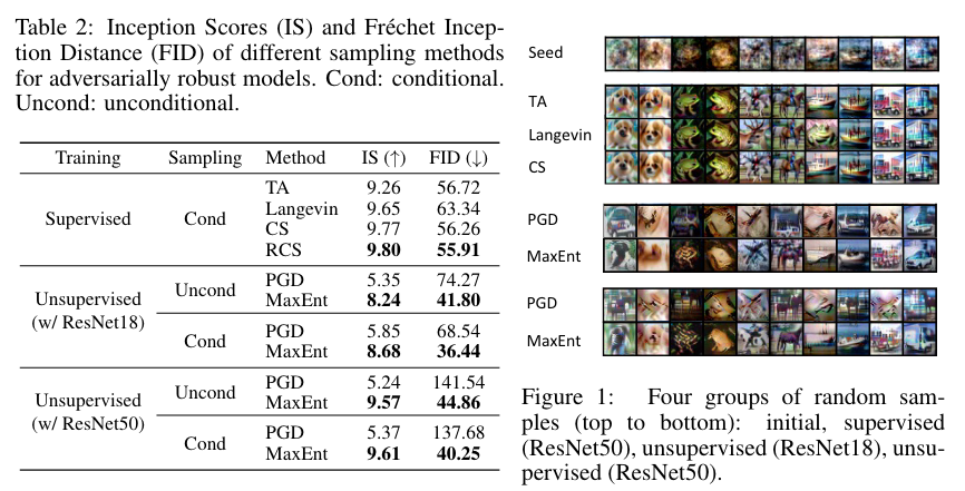
Experiments