선형 회귀 모델의 구현방법
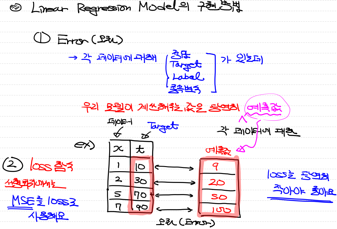
11.29 복습
위의 상태로 진행되게 됩니다.
이때 맨밑 그림에서 이상치들이 발생합니다.
데이터 전처리
- 결측치 처리
- 이상치 처리
- 정규화 처리
순서대로 진행하는것이 좋습니다.
이상치
모델이 회귀모델 즉 조건부 평균을 구하는 것인데 이런 이상치가 발생하게되면 모델이 좋아지지 않는다.
독립변수(Temp) => 여기서 발생하는 편차가 큰 값은 => 지대점
종속변수(Ozone) => 여기서 발생하는 편차가 큰 값 => 이상치(outlier)
이상치 제거 방법
- Tukey's Fense 방식 => 사분위를 이용
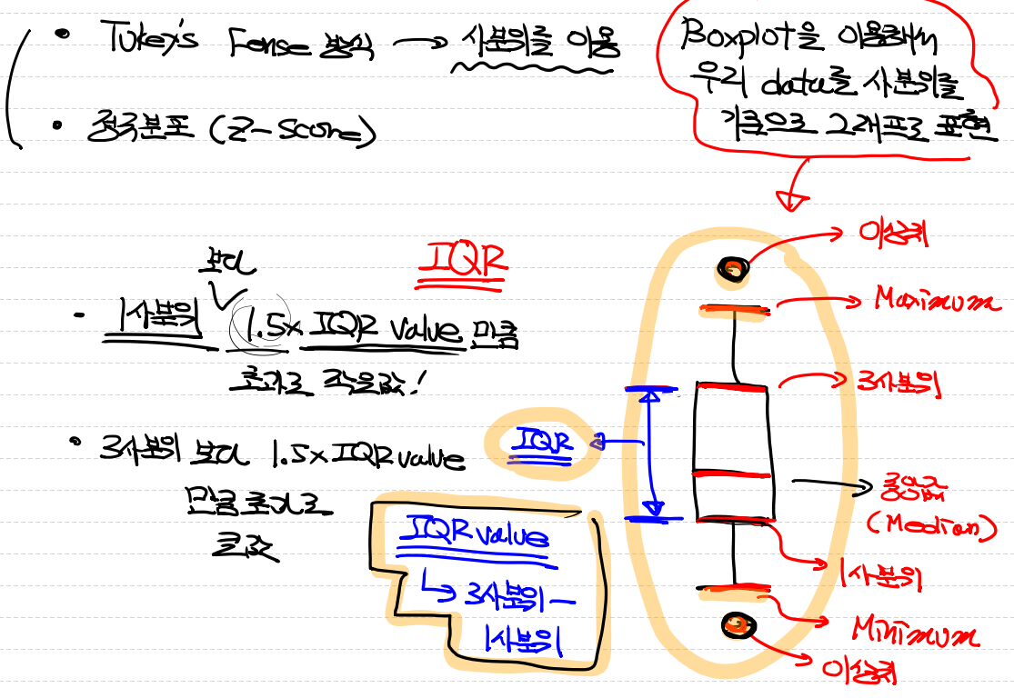
boxplot을 그린 후 maximum보다 더 크거나 minimum 더 작으면 이상치로 판단한다. - 정규분포(Z -score)
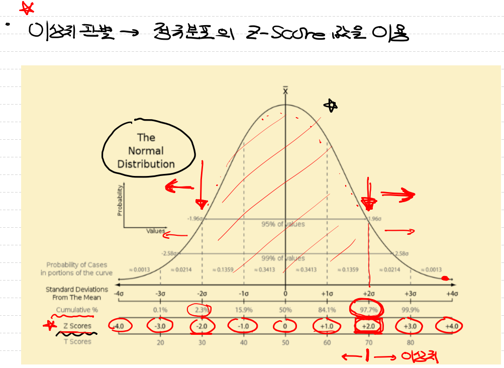
Z-score는 각 포인터들 평균과의 거리가 얼마나 멀어져있는지 확인을 한 후 +-2이 넘어가면 이상치로 판단한다.
이상치를 모두 제거한다고 하더라도 우리가 원하는 모델이 완성되지 않았습니다. 왜 why?
정규화를 진행하지 않았기때문입니다.
정규화
정규화를 해야하는 이유
- feature scale을 조정한다.
- 학습속도를 향상시켜준다.
- 특정 feature에 가중치가 더 부여되는 overfitting을 피할 수 있다.
- 수치안정성(계산의 정확도가 높아진다)
- 거리기반 알고리즘들이 존재하는데 이 알고리즘을 사용할때는 필수적으로 사용해야한다.
정규화 방법
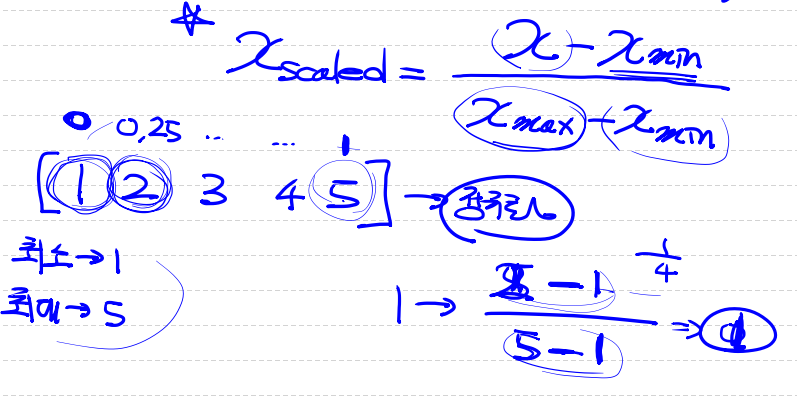
1. Min-Max normalization(scaling)
- 정규화를 하는 가장 일반적인 방법이다.
- 모든 feature에 대해 최소 0 ~ 최대 1의 값을 설정하는 것이다.
- 이상치에 민감하다.
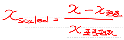
2. Standardization(Z-score Nomalization) - 평균 및 표준편차와의 관계측면에서 데이터 포인트를 설명하는 방법이다.
- 이상치에 둔감하다
파이썬 구현
Ozone 데이터 실습 예제
python 직접 구현
# python 직접구현
import numpy as np
import pandas as pd
import matplotlib.pyplot as plt
# 수치미분코드
def numerical_derivative(f, x): # x가 다변수함수이기때문에 2개가 들어가야함
delta_x =1e-4
derivative_x = np.zeros_like(x) # [0.0, 0.0]
it = np.nditer(x, flags=['multi_index'])
while not it.finished:
idx = it.multi_index # 현재의 index를 추출 => tuple형태로 리턴
tmp = x[idx] # 현재 index의 값을 일단 잠시 보존해요.
# 밑에서 이 값을 변경해서 중앙차분 값을 계산해야함
# 그런데 우리 편미분을 해야하는데 다음 변수 편미분을 할때에
# 원래값으로 복원해야 정상적으로 진행되기 때문에
# 이 값을 잠시 보관했다가 원상태로 복구해야함
x[idx] = tmp + delta_x
fx_plus_delta_x = f(x) # f(x + delta_x)
x[idx] = tmp - delta_x
fx_minus_delta_x = f(x)
derivative_x[idx] = (fx_plus_delta_x - fx_minus_delta_x) / (2 * delta_x)
x[idx] = tmp
it.iternext()
return derivative_x
# Raw Data Loading
df = pd.read_csv('/content/drive/MyDrive/Colab Notebooks/ML/data/ozone/ozone.csv')
# display(df)
# 그러면 먼저 사용할 데이터를 추출해보자
training_data = df[['Temp', 'Ozone']]
# display(training_data) # 153 rows × 2 columns
# 삭제해서 사용해보자
training_data = training_data.dropna(how='any')
# display(training_data) # 116 rows × 2 columns
# Training Data Set
x_data = training_data['Temp'].values.reshape(-1,1)
t_data = training_data['Ozone'].values.reshape(-1,1)
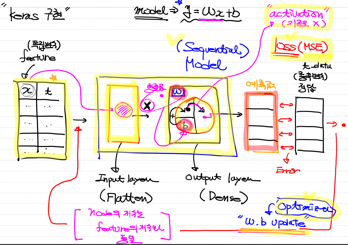
# Model을 만들어야하는데.. y = Wx + b
W = np.random.rand(1,1)
b = np.random.rand(1)
# loss function(MSE)
def loss_func(input_data):
input_w = input_data[0]
input_b = input_data[1]
y = np.dot(x_data, input_w) + input_b
# loss 함수는 mse를 리턴해줌
return np.mean(np.power((t_data - y), 2))
# 예측작업을 해야 해요! 그래서 예측을 해주는 함수를 하나 정의
def predict(x): # 입력값 x
return np.dot(x, W) + b
# 하이퍼파라미터 설정
# epoch => 전체를 한번 도는것
# lenaring rate 정의
learning_rate = 1e-4
# 학습을 진행
for step in range(300000):
# 현재 W는 2차원, b는 1차원입니다
# 그런데 이게 loss함수 안으로 들어갈때는 1차원 안에 두 값이
# 순서대로 들어가 있어야 한다
# ravel() 1차원으로 펴주는 함수
# concatenate로 둘의 1차원 값을 합쳐줌.
# 어디로 붙일지 지정을 해줘야함.
# 축을 설정해주어야함.
# 입력인자를 설정해주었음.
input_param = np.concatenate((W.ravel(), b.ravel()), axis=0)
derivative_result = learning_rate * numerical_derivative(loss_func, input_param)
# 이제 입력인자를 미분해주어야함.
# 미분함수에 loss함수를 넣고, 입력인자를 넣어줌.
# learning rate를 설정하고 함수 결과를 선언해줌
W = W - derivative_result[0].reshape(-1,1)
b = b - derivative_result[1]
# 확인 작업
if step % 30000 == 0:
print(f'W: {W}, b: {b}, loss: {loss_func(input_param)}')
# 학습종료 후 예측
# 온도가 62도일때 Ozone량은 얼마?
print(predict(np.array([[62]]))) # [[16.88607015]]
# 이거 맞는거야???
# 그래프로 확인해 보아요!
# (독립변수 1개니까 2차원 평면에 모델을 그릴수 있어요!)
# 데이터를 2차원 평면에 찍어보아요!
plt.scatter(x_data, t_data) # [[16.88607015]]
# 우리 모델을 그려보아요!
plt.plot(x_data, x_data*W.ravel() + b, color='r')
plt.show()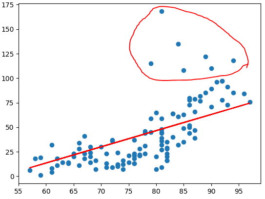
Tensorflow 구현
# 같은 내용을 이제 Tensorflow Keras를 이용해서 구현!

import numpy as np
import pandas as pd
import matplotlib.pyplot as plt

from tensorflow.keras.models import Sequential
from tensorflow.keras.layers import Flatten, Dense
from tensorflow.keras.optimizers import SGD

# Raw Data Loading
df = pd.read_csv('/content/drive/MyDrive/Colab Notebooks/ML/data/ozone/ozone.csv')

training_data = df[['Temp', 'Ozone']]

# 이렇게 데이터를 가져온 후 당연히 데이터 전처리를 해야 해요!
# 1. 결측치 처리!
training_data = training_data.dropna(how='any')

# Training Data Set 준비
x_data = training_data['Temp'].values.reshape(-1,1)
t_data = training_data['Ozone'].values.reshape(-1,1)

# Model 생성
model = Sequential()

model.add(Flatten(input_shape=(1,)))

output_layer = Dense(units=1,
                     activation='linear')

model.add(output_layer)

# model 설정
model.compile(optimizer=SGD(learning_rate=1e-4),
              loss='mse')

# model 학습
model.fit(x_data,
          t_data,
          epochs=2000,
          verbose=0)

# 학습이 끝났으니 예측을 해 보아요!
print(model.predict(np.array([[62]])))  # [[39.92358]]

# 그래프로 확인해 보아요!
# W와 b가 필요해요!
weights, bias = output_layer.get_weights()

# 데이터를 2차원 평면에 찍어보아요!
plt.scatter(x_data, t_data)
# 우리 모델을 그려보아요!
plt.plot(x_data, x_data*weights + bias, color='r')
plt.show()   # [[39.92358]]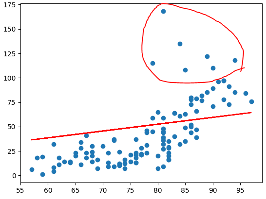
sklearn 구현
# 정답(?)을 확인하기 위해 sklearn 구현을 해 보아요!

import numpy as np
import pandas as pd
import matplotlib.pyplot as plt
from sklearn import linear_model


# Raw Data Loading
df = pd.read_csv('/content/drive/MyDrive/Colab Notebooks/ML/data/ozone/ozone.csv')

training_data = df[['Temp', 'Ozone']]

# 이렇게 데이터를 가져온 후 당연히 데이터 전처리를 해야 해요!
# 1. 결측치 처리!
training_data = training_data.dropna(how='any')

# Training Data Set 준비
x_data = training_data['Temp'].values.reshape(-1,1)
t_data = training_data['Ozone'].values.reshape(-1,1)

# Model 생성
sklearn_model = linear_model.LinearRegression()

# Model 학습
sklearn_model.fit(x_data, t_data)

# W와 b를 알아야지 나중에 그래프를 그릴 수 있겠죠.
weights = sklearn_model.coef_
bias = sklearn_model.intercept_

# 예측을 해 보아요!
print(sklearn_model.predict(np.array([[62]])))  # [[3.58411393]]

# 데이터를 2차원 평면에 찍어보아요!
plt.scatter(x_data, t_data)
# 우리 모델을 그려보아요!
plt.plot(x_data, x_data*weights + bias, color='r')
plt.show()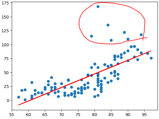
이상치 제거
# Tukey's Fence 방식으로 이상치를 검출해보아요!

import numpy as np
import matplotlib.pyplot as plt

data = np.array([1,2,3,4,5,6,7,8,9,10,11,12,13,14,22.1])

fig = plt.figure()

fig_1 = fig.add_subplot(1,2,1)  # 1행 2열의 첫번째
fig_2 = fig.add_subplot(1,2,2)  # 1행 2열의 두번째

print(np.median(data))  # 8.0
print(np.percentile(data,25))  # 4.5
print(np.percentile(data,75))  # 11.5

# IQR value
iqr_value = np.percentile(data,75) - np.percentile(data,25)
print(iqr_value)  # 7.0

upper_fence = np.percentile(data,75) + 1.5 * iqr_value
print(upper_fence)  # 22.0
lower_fence = np.percentile(data,25) - 1.5 * iqr_value
print(lower_fence)  # -6.0

# 아하!! 이렇게 tukey fence방식을 이용하면 이상치를 구분하는
# 기준선을 알아낼 수 있네요!

# 내가 가지고 있는 데이터에 대해 이상치를 출력해보세요!
# boolean indexing을 이용해요!

print(data[(data > upper_fence) | (data < lower_fence)])  # [22.1]

# 데이터를 정제하는게 목적이예요. 이상치를 제거하는게 목적!
result_data = data[(data <= upper_fence) & (data >= lower_fence)]
print(result_data)

fig_1.set_title('Original Data')
fig_1.boxplot(data)

fig_2.set_title('Remove Outlier Data')
fig_2.boxplot(result_data)

plt.tight_layout()
plt.show()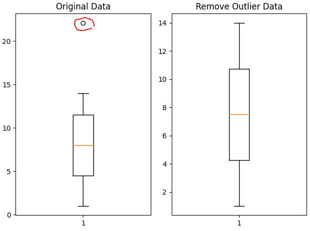
# 정규분포(Z-score)를 이용한 이상치 구별방식
# 이 방식을 이용하려면
# 기본적으로 우리 데이터를 정규분포화 시켜서 우리 데이터에 대한
# z-score값을 각각 구해야 되요!
# 그리고 기준치를 설정한 다음 그 기준치를 넘는 데이터를 이상치로 판별

from scipy import stats

data = np.array([1,2,3,4,5,6,7,8,9,10,11,12,13,14,22.1])

zscore_threshold = 2.0 # 일반적으로 2.0을 많이 사용.

# print(np.abs(stats.zscore(data)) > zscore_threshold)
outlier = data[np.abs(stats.zscore(data)) > zscore_threshold] # [22.1]

# 이상치를 제거한 결과
print(data[np.isin(data,outlier, invert=True)])
# [ 1.  2.  3.  4.  5.  6.  7.  8.  9. 10. 11. 12. 13. 14.
from scipy import stats
# 데이터는 공통으로 사용하니 먼저 사용하는 데이터 정제부터 하고
# 각각 구현하는게 좋을 듯 싶어요!
# Raw Data Loading
df = pd.read_csv('/content/drive/MyDrive/Colab Notebooks/ML/data/ozone/ozone.csv')
training_data = df[['Temp', 'Ozone']]
# 이렇게 데이터를 가져온 후 당연히 데이터 전처리를 해야 해요!
# 1. 결측치 처리!
training_data = training_data.dropna(how='any')
# 2. 이상치 처리!
zscore_threshold = 1.8
outlier = training_data['Ozone'][np.abs(stats.zscore(training_data['Ozone'].values)) > zscore_threshold]
# print(outlier)
# 이상치를 제거한 결과를 얻어야 해요!
# 내가 가진 DataFrame에서 이상치를 제거하면 되요!
training_data = training_data.loc[np.isin(training_data['Ozone'],outlier, invert=True)]
# Training Data Set 준비
x_data = training_data['Temp'].values.reshape(-1,1)
t_data = training_data['Ozone'].values.reshape(-1,1)
이상치 제거 후 구현
python 직접 구현
# Python 직접구현
import numpy as np
import pandas as pd
import matplotlib.pyplot as plt
## 수치미분 코드
def numerical_derivative(f,x):
# f : 미분하려고하는 다변수 함수
# x : 모든 변수를 포함하는 ndarray [1.0 2.0]
# 리턴되는 결과는 [8.0 15.0]
delta_x = 1e-4
derivative_x = np.zeros_like(x) # [0.0 0.0]
it = np.nditer(x, flags=['multi_index'])
while not it.finished:
idx = it.multi_index # 현재의 index를 추출 => tuple형태로 리턴.
tmp = x[idx] # 현재 index의 값을 일단 잠시 보존해야해요!
# 밑에서 이 값을 변경해서 중앙차분 값을 계산해야 해요!
# 그런데 우리 편미분해야해요. 다음 변수 편미분할때
# 원래값으로 복원해야 편미분이 정상적으로 진행되기 때문에
# 이값을 잠시 보관했다가 원상태로 복구해야 해요!
x[idx] = tmp + delta_x
fx_plus_delta_x = f(x) # f(x + delta_x)
x[idx] = tmp - delta_x
fx_minus_delta_x = f(x) # f(x - delta_x)
derivative_x[idx] = (fx_plus_delta_x - fx_minus_delta_x) / (2 * delta_x)
x[idx] = tmp
it.iternext()
return derivative_x
# Model을 만들어야 하는데.. y = Wx + b
W = np.random.rand(1,1)
b = np.random.rand(1)
# loss function(MSE)
def loss_func(input_data):
input_w = input_data[0]
input_b = input_data[1]
y = np.dot(x_data, input_w) + input_b
return np.mean(np.power((t_data-y),2))
# 모델이 완성된 후 예측하는 함수를 하나 만들어요!
def predict(x):
return np.dot(x, W) + b
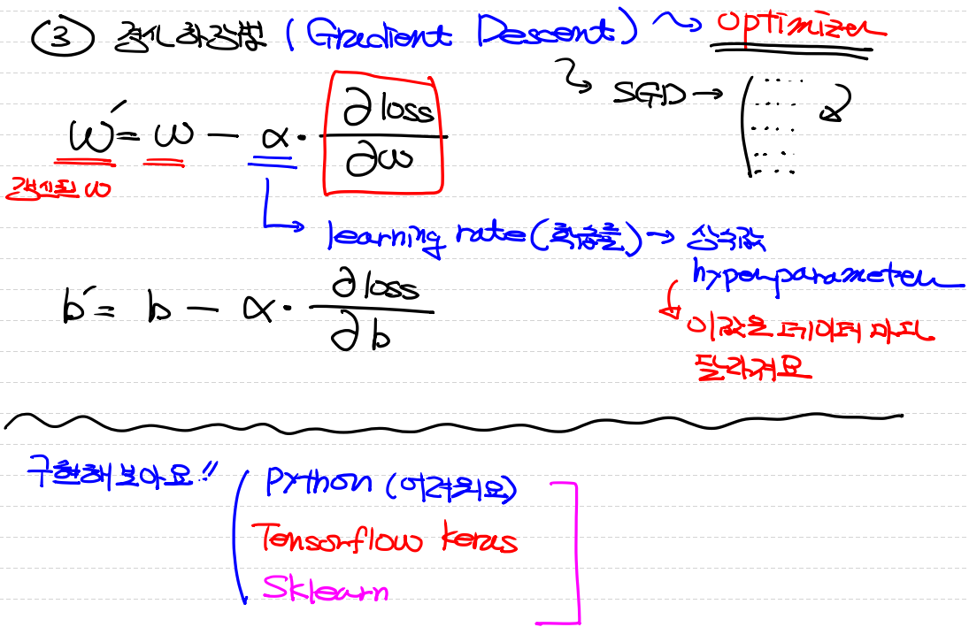
# learning rate 정의(hyperparameter)
learning_rate = 1e-4
# 학습진행
for step in range(300000):
input_param = np.concatenate((W.ravel(), b.ravel()), axis=0)
derivative_result = learning_rate * numerical_derivative(loss_func, input_param)
W = W - derivative_result[0].reshape(-1,1)
b = b - derivative_result[1]
if step % 30000 == 0:
print(f'W : {W}, b : {b}, loss : {loss_func(input_param)}')
# 학습종료 후 예측
# 온도가 62도일때 Ozone량은 얼마?
print(predict(np.array([[62]]))) # [[15.51232223]]Tensorflow 구현
# 같은 내용을 이제 Tensorflow Keras를 이용해서 구현!

from tensorflow.keras.models import Sequential
from tensorflow.keras.layers import Flatten, Dense
from tensorflow.keras.optimizers import SGD

# Model 생성
model = Sequential()

model.add(Flatten(input_shape=(1,)))

output_layer = Dense(units=1,
                     activation='linear')

model.add(output_layer)

# model 설정
model.compile(optimizer=SGD(learning_rate=1e-4),
              loss='mse')

# model 학습
model.fit(x_data,
          t_data,
          epochs=2000,
          verbose=0)

# 학습이 끝났으니 예측을 해 보아요!
print(model.predict(np.array([[62]])))  # [[37.21062]]

# 그래프로 확인해 보아요!
# W와 b가 필요해요!
weights, bias = output_layer.get_weights()
sklearn 구현
# 정답(?)을 확인하기 위해 sklearn 구현을 해 보아요!
import numpy as np
import pandas as pd
import matplotlib.pyplot as plt
from sklearn import linear_model
# Model 생성
sklearn_model = linear_model.LinearRegression()
# Model 학습
sklearn_model.fit(x_data, t_data)
# 예측을 해 보아요!
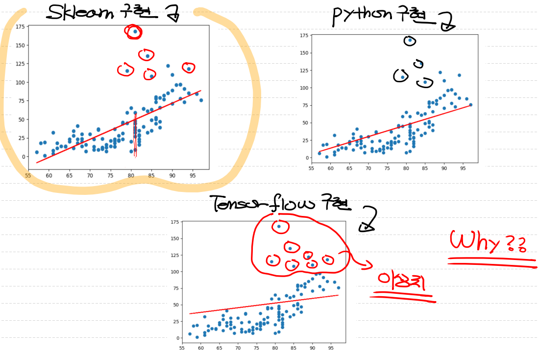
print(sklearn_model.predict(np.array([[62]]))) # [[4.51299041]]그래프로 확인해보기
####### 결과를 그래프로 확인해 보아요! #########

fig = plt.figure()

fig_python = fig.add_subplot(1,3,1)
fig_tensorflow = fig.add_subplot(1,3,2)
fig_sklearn = fig.add_subplot(1,3,3)

fig_python.set_title('python')
fig_tensorflow.set_title('tensorflow')
fig_sklearn.set_title('sklearn')

fig_python.scatter(x_data, t_data)
fig_python.plot(x_data, x_data*W.ravel() + b, color='r')

fig_tensorflow.scatter(x_data, t_data)
fig_tensorflow.plot(x_data, x_data*weights + bias, color='b')

fig_sklearn.scatter(x_data, t_data)
fig_sklearn.plot(x_data,
                 x_data*sklearn_model.coef_ + sklearn_model.intercept_,
                 color='g')

plt.tight_layout()
plt.show()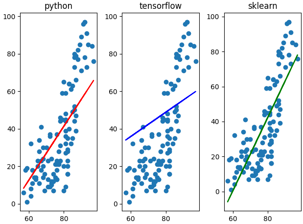

XD