[AI] PyTorch : 3. Multivariable Linear Regression

NewPlus·2022년 6월 27일

목록 보기

3/11

2022.06.27 연구실 공부(PyTorch). 'PyTorch로 시작하는 딥 러닝 입문'< 이 글은 이 책의 내용을 요약 정리한 것임.>(내 저작물이 아니고 저 위 링크에 있는 것이 원본임)
03-03 Multivariable Linear Regression

Summary

Data Definition
파이토치로 구현하기
벡터와 행렬 연산으로 바꾸기
행렬 연산을 고려하여 파이토치로 구현하기

1. Data Definition

훈련 데이터(독립변수 x의 개수가 4개임 -> 최종점수 예측하는 모델)
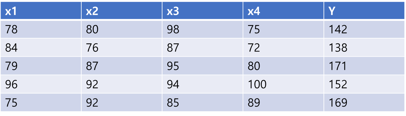
수식

2. 파이토치로 구현하기

기본 임포트 및 랜덤 시드 고정

import torch
import torch.nn as nn
import torch.nn.functional as F
import torch.optim as optim

torch.manual_seed(1)

식에서 x의 개수가 4개 이므로 x_train도 4개 선언

# 훈련 데이터
x1_train = torch.FloatTensor([[78], [84], [79], [96], [75]])
x2_train = torch.FloatTensor([[80], [76], [87], [92], [92]])
x3_train = torch.FloatTensor([[98], [87], [95], [94], [85]])
x4_train = torch.FloatTensor([[75], [72], [80], [100], [89]])
y_train = torch.FloatTensor([[142], [138], [171], [152], [169]])

가중치 w(x의 개수에 맞게 4개 선언)와 편향 b를 선언

# 가중치 w와 편향 b 초기화
w1 = torch.zeros(1, requires_grad=True)
w2 = torch.zeros(1, requires_grad=True)
w3 = torch.zeros(1, requires_grad=True)
w4 = torch.zeros(1, requires_grad=True)
b = torch.zeros(1, requires_grad=True)

Hypothesis, Cost Function(torch.mean 제곱), Optimizer 선언 -> 경사하강법 1000회 반복(epoch) -> 결과를 100단위로 출력

# optimizer 설정
optimizer = optim.SGD([w1, w2, w3, w4, b], lr=1e-5)

nb_epochs = 1000
for epoch in range(nb_epochs + 1):

    # H(x) 계산
    hypothesis = x1_train * w1 + x2_train * w2 + x3_train * w3 + x4_train * w4 + b
    # cost 계산
    cost = torch.mean((hypothesis - y_train) ** 2)

    # cost로 H(x) 개선
    optimizer.zero_grad()
    cost.backward()
    optimizer.step()

    # 100번마다 로그 출력
    if epoch % 100 == 0:
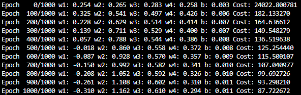
        print('Epoch {:4d}/{} w1: {:.3f} w2: {:.3f} w3: {:.3f} w4: {:.3f} b: {:.3f} Cost: {:.6f}'.format(
            epoch, nb_epochs, w1.item(), w2.item(), w3.item(), w4.item(), b.item(), cost.item()
        ))

1000회 출력(100 epoch마다 출력)

3. 벡터와 행렬 연산으로 바꾸기

위 처럼 일일이 선언할 경우 x의 개수가 1000개일 경우에는 x,w 선언이 어렵다
행렬의 곱셈 연산 혹은 벡터의 내적을 통해 이 문제를 해결한다.
이는 곧 1 x 7 + 2 x 9 + 3 x 11 = 58이 된다.

3-1. 벡터 연산으로 이해하기

위 식을 다음 과 같이 내적으로 표현할 수 있다.
이제 다음과 같이 두 개의 변수로 표시된다.

3-2. 행렬 연산으로 이해하기

행 : 샘플(Sample), 열 : 특성(Feature)
Sample은 현재 5개, Feature는 4개이므로 (Sample * Feature) = 20개의 원소를 갖는 행렬 X를 표현하면 다음과 같다.
여기에 가중치를 원소로 하는 벡터 W를 곱하면 다음과 같다.
위 행렬 곱을 식으로 간략히 나타내면 다음과 같다.

4. 행렬 연산을 고려하여 파이토치로 구현하기

훈련 데이터 행렬 형식으로 선언

# 훈련 데이터
x_train = torch.FloatTensor([[78, 80, 98, 75],
                            [84, 76, 87, 72],
                            [79, 87, 95, 80],
                            [96, 92, 94, 100],
                            [75, 92, 85, 89]])
y_train = torch.FloatTensor([[142], [138], [171], [152], [169]])

행렬 곱 연산을 위해 크기가 맞는지 확인한다.

print(x_train.shape)
print(y_train.shape)

torch.Size([5, 4])
torch.Size([5, 1])

각 행렬이 (5 x 4), (5 x 1)이므로 가중치 행렬을 초기화할 때 크기를 (4 x 1)로 맞춰준다.

# 가중치와 편향 선언
W = torch.zeros((4, 1), requires_grad=True)
b = torch.zeros(1, requires_grad=True)

Hypothesis, Cost Function(torch.mean 제곱), Optimizer 선언 -> 경사하강법 1000회 반복(epoch) -> 결과를 100단위로 출력

# optimizer 설정
optimizer = optim.SGD([W, b], lr=1e-5)

nb_epochs = 1000
for epoch in range(nb_epochs + 1):

    # H(x) 계산
    # 편향 b는 브로드 캐스팅되어 각 샘플에 더해집니다.
    hypothesis = x_train.matmul(W) + b

    # cost 계산
    cost = torch.mean((hypothesis - y_train) ** 2)

    # cost로 H(x) 개선
    optimizer.zero_grad()
    cost.backward()
    optimizer.step()
    # 100번마다 로그 출력
    if epoch % 100 == 0:
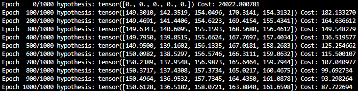
        print('Epoch {:4d}/{} hypothesis: {} Cost: {:.6f}'.format(
            epoch, nb_epochs, hypothesis.squeeze().detach(), cost.item()
        ))